Mastering Classification Metrics: A Deep Dive from F1-Score to AUC-ROC

When building AI systems for classification tasks—whether to detect spam, diagnose cancer, or prevent fraud—evaluating your model correctly is just as important as training it.

In classification problems, it’s tempting to focus on accuracy, but that alone can be misleading, especially when dealing with imbalanced datasets. An imbalanced dataset is one where the classes are not represented equally; for example, in a spam detection scenario, you might have 90% "ham" (non-spam) emails and only 10% "spam" emails. This guide walks through the core evaluation metrics you need to understand in such contexts, with a deep dive into F1-score and related threshold-based metrics, and provides a seamless transition into AUC-ROC—a more nuanced way to evaluate your model’s performance across all thresholds.

📩 Let’s Take Spam Classification as an Example

Imagine you train a model to classify emails as spam (the positive class) or ham (not spam, the negative class). You want to know: How well does the model perform this classification task, particularly in identifying spam? This is where metrics like the F1-score, Precision, Recall, and AUC-ROC become essential tools for assessment.

The F1-Score: A Harmonious Blend of Precision and Recall

The F1-score stands out as a crucial metric in classification tasks, particularly when an imbalance exists between classes or when the consequences of false positives and false negatives are not symmetrical. It is defined as the harmonic mean of two other fundamental metrics: Precision and Recall. This choice of the harmonic mean is deliberate; unlike a simple arithmetic average, the harmonic mean heavily penalizes low values. Consequently, for the F1-score to be high, both precision and recall must be reasonably high. If either precision or recall is poor, the F1-score will also be low, reflecting a more nuanced assessment of the model's performance than accuracy alone might provide.

The formula for the F1-score is:

F1-Score = 2 * (Precision * Recall) / (Precision + Recall)

To truly understand the F1-score, we must first delve into Precision and Recall, and the foundational concepts of True Positives, False Positives, True Negatives, and False Negatives, often visualized using a confusion matrix.

Defining the Core Components: TP, FP, FN, TN and the Confusion Matrix

Imagine we are building a model to classify emails as either "spam" (positive class) or "ham" (not spam, negative class). After the model makes its predictions on a set of emails, we can categorize each prediction into one of four outcomes. These outcomes are typically summarized in a confusion matrix:

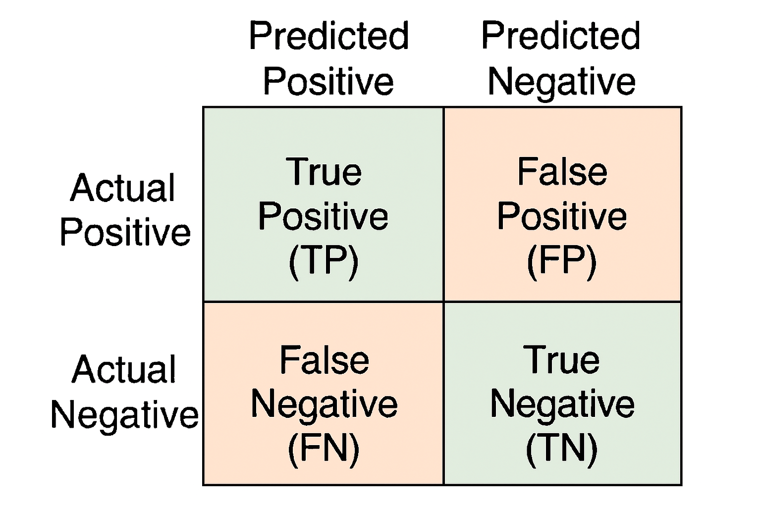
Figure 1: A typical 2x2 Confusion Matrix illustrating the four possible outcomes of a binary classification.

As shown in the confusion matrix, the four outcomes are:

• True Positive (TP): The email was actually spam, and the model correctly predicted it as spam. This is a desired outcome – the model successfully identified a spam email.
• False Positive (FP): The email was actually ham (not spam), but the model incorrectly predicted it as spam. This is also known as a Type I error. For instance, an important work email mistakenly sent to the spam folder.
• False Negative (FN): The email was actually spam, but the model incorrectly predicted it as ham (i.e., it missed the spam). This is also known as a Type II error. For instance, a phishing email landing in the inbox, appearing legitimate.
• True Negative (TN): The email was actually ham, and the model correctly predicted it as ham. This is also a desired outcome – the model correctly identified a legitimate email.

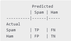
Figure 2: Truth table for "Spam" and "Ham" in our example.

Precision: The Purity of Positive Predictions

Precision addresses the question: "Of all the emails that the model flagged as spam, how many were actually spam?" It measures the accuracy of the positive predictions. A high precision means that when the model predicts an email is spam, it is very likely to be correct. This is particularly important in scenarios where a false positive is costly. For example, if an email filter has low precision, users might miss important legitimate emails that are incorrectly classified as spam.

The formula for Precision is:

Precision = TP / (TP + FP)

Example: Calculating Precision

Let's say our email classification model processes 100 emails. After evaluation, we find:

• True Positives (TP) = 30 (30 spam emails correctly identified as spam)
• False Positives (FP) = 5 (5 ham emails incorrectly identified as spam)
• True Negatives (TN) = 60 (60 ham emails correctly identified as ham)
• False Negatives (FN) = 5 (5 spam emails missed and identified as ham)

First, let's identify the components for the precision calculation:

• TP = 30
• FP = 5

The total number of emails predicted as spam by the model is

TP + FP = 30 + 5 = 35.

Now, we calculate precision:

Precision = 30 / (30 + 5) = 30 / 35 = 0.8571 (or 85.71%)

This means that 85.71% of the emails our model flagged as spam were indeed spam. The remaining 14.29% were legitimate emails incorrectly classified.

Recall (Sensitivity): Catching All Positives

Recall, also known as Sensitivity or True Positive Rate (TPR), answers the question: "Of all the actual spam emails that existed in the dataset, how many did the model correctly identify?" It measures the model's ability to find all relevant instances of the positive class. High recall is crucial when missing a positive instance (a false negative) is very costly. For example, in medical diagnosis for a serious disease, high recall is paramount because failing to detect the disease in a patient who has it can have severe consequences.

The formula for Recall is:

Recall = TP / (TP + FN)

Example: Calculating Recall

Using the same email classification scenario and results as above:

• True Positives (TP) = 30 (30 spam emails correctly identified as spam)
• False Positives (FP) = 5
• True Negatives (TN) = 60
• False Negatives (FN) = 5 (5 spam emails missed and identified as ham)

For recall, the components are:

• TP = 30
• FN = 5

The total number of actual spam emails in the dataset is

TP + FN = 30 + 5 = 35.

Now, we calculate recall:

Recall = 30 / (30 + 5) = 30 / 35 = 0.8571 (or 85.71%)

This means our model successfully identified 85.71% of all the spam emails present in the dataset. It missed 14.29% of the actual spam.

Bringing it Together: Calculating the F1-Score

Now that we have calculated Precision (0.8571) and Recall (0.8571) for our email classification example, we can calculate the F1-score:

F1-Score = 2 * (Precision * Recall) / (Precision + Recall)
F1-Score = 2 * (0.8571 * 0.8571) / (0.8571 + 0.8571)
F1-Score = 2 * (0.7346) / (1.7142)
F1-Score = 1.4692 / 1.7142
F1-Score = 0.8571 (or 85.71%)

In this particular example, since Precision and Recall are equal, the F1-score is also the same. However, this is not always the case. Consider a scenario where Precision is high but Recall is low, or vice-versa.

Example 2: F1-Score with differing Precision and Recall

Suppose a different model has:

• Precision = 0.90 (90%)
• Recall = 0.60 (60%)

F1-Score = 2 * (0.90 * 0.60) / (0.90 + 0.60)
F1-Score = 2 * (0.54) / (1.50)
F1-Score = 1.08 / 1.50
F1-Score = 0.72 (or 72%)

The arithmetic mean of 0.90 and 0.60 would be (0.90 + 0.60) / 2 = 0.75. The F1-score (0.72) is lower than the arithmetic mean, illustrating how the harmonic mean pulls the score towards the lower value, providing a more conservative and often more realistic measure of performance when there's a trade-off between precision and recall.

The F1-score provides a single metric that balances the concerns of precision and recall, making it a popular choice for evaluating classification models, especially when dealing with imbalanced datasets where one class is much more frequent than the other.

Variants of F1-Score for Multi-Class Classification

When dealing with classification problems that involve more than two classes (multi-class classification), the F1-score needs to be adapted. Two common approaches for this are the Macro F1 and Weighted F1 scores.

Macro F1-Score (or Macro-Averaged F1-Score):

The Macro F1-score calculates the F1-score independently for each class and then takes the simple arithmetic average of these scores. This method treats all classes equally, regardless of their frequency in the dataset (i.e., their support).

Calculation Steps:

1. For each class i in your multi-class problem, calculate its individual F1-score (F1_i). This involves determining the TP, FP, and FN specific to that class (often by treating it as a one-vs-rest scenario).
2. Sum up all the individual F1-scores.
3. Divide the sum by the total number of classes.

Macro F1 = (F1_class1 + F1_class2 + ... + F1_classN) / N (where N is the number of classes)

When to use Macro F1:
Macro F1 is useful when you want to assess how well the model performs on each class on average, without giving more importance to larger classes. If your goal is to have good performance across all classes, even the rare ones, Macro F1 is a good indicator. However, it can be sensitive to poor performance on a single class, even if that class is infrequent.

Example: Macro F1 Calculation

Suppose we have a 3-class classification problem (Class A, Class B, Class C) and our model achieves the following individual F1-scores for each class:

• F1-score for Class A = 0.90
• F1-score for Class B = 0.80
• F1-score for Class C = 0.60 (perhaps Class C is a rare or difficult class)

Macro F1 = (0.90 + 0.80 + 0.60) / 3
Macro F1 = 2.30 / 3
Macro F1 ≈ 0.7667

This score gives equal weight to the performance on Class C, even if it was much smaller than A or B.

Weighted F1-Score (or Weighted-Averaged F1-Score):

The Weighted F1-score also calculates the F1-score for each class independently, but then it takes a weighted average of these scores. The weight for each class's F1-score is its support, which is the number of true instances of that class in the dataset.

Calculation Steps:

1. For each class i, calculate its individual F1-score (F1_i).
2. For each class i, determine its support (S_i), which is the number of actual instances belonging to that class.
3. Multiply each class's F1-score by its support: F1_i * S_i.
4. Sum these weighted scores.
5. Divide the sum by the total number of instances in the dataset (which is the sum of all supports).

Weighted F1 = (F1_class1S_class1 + F1_class2S_class2 + ... + F1_classN*S_classN) / (S_class1 + S_class2 + ... + S_classN)

When to use Weighted F1:
Weighted F1 is useful when you want an F1-score that accounts for class imbalance. It gives more importance to the F1-scores of the more frequent classes. If performing well on the majority classes is more critical, or if you want a score that better reflects the overall performance on the dataset considering its class distribution, Weighted F1 is more appropriate. It can mask poor performance on minority classes if those classes have very low support.

Example: Weighted F1 Calculation

Continuing with our 3-class problem, let's assume the following supports (number of actual instances):

• Support for Class A (S_A) = 100 instances
• Support for Class B (S_B) = 50 instances
• Support for Class C (S_C) = 10 instances

And the individual F1-scores were:

• F1-score for Class A = 0.90
• F1-score for Class B = 0.80
• F1-score for Class C = 0.60

Total instances = 100 + 50 + 10 = 160
Weighted F1 = (0.90 * 100 + 0.80 * 50 + 0.60 * 10) / (100 + 50 + 10)
Weighted F1 = (90 + 40 + 6) / 160
Weighted F1 = 136 / 160
Weighted F1 = 0.85

Notice that the Weighted F1 (0.85) is higher than the Macro F1 (0.7667). This is because Class A, which has a high F1-score (0.90), also has the highest support, thus contributing more to the weighted average. The lower F1-score of Class C (0.60) has less impact on the Weighted F1 because of its small support.

Choosing between Macro F1 and Weighted F1 depends on the specific goals of your classification task and whether you prioritize consistent performance across all classes or overall performance biased towards the majority classes. Often, it is insightful to report both, along with per-class F1-scores, to get a complete picture of the model's behavior.

The Pitfalls of Accuracy: Why It Can Be Deceptive

Accuracy is often the first metric that comes to mind when evaluating a classification model. It simply measures the proportion of total predictions that the model got right. The formula is straightforward:

Accuracy = (True Positives + True Negatives) / (Total Number of Instances)

Where:

• True Positives (TP): Correctly predicted positive instances.
• True Negatives (TN): Correctly predicted negative instances.
• Total Number of Instances: The sum of all instances (TP + TN + False Positives (FP) + False Negatives (FN)).

While intuitively appealing, relying solely on accuracy can be dangerously misleading, especially when dealing with imbalanced datasets – datasets where one class is far more prevalent than others (as defined in our introduction, e.g., 90% "ham" and 10% "spam" in email filtering, or 990 healthy individuals versus 10 with cancer in medical screening).

Let's illustrate this with a critical example: a model designed for cancer screening.

Suppose we have the following scenario:

• Total people screened: 1000
• Actual cancer cases (positive class): 10 people
• Healthy people (negative class): 990 people

Now, imagine our model is poorly designed or, in an extreme case, simply predicts every single person as healthy. Let's analyze the outcomes:

• The model predicts all 1000 people as healthy.
• Since there are 990 healthy people, the model correctly identifies them as healthy. These are True Negatives (TN) = 990.
• Since there are 10 people with cancer, and the model predicts them as healthy, it incorrectly classifies them. These are False Negatives (FN) = 10 (the model missed all cancer cases).
• The model did not predict anyone as having cancer, so there are no True Positives (TP) = 0.
• Similarly, since no one was predicted as having cancer, there are no instances where a healthy person was wrongly flagged as having cancer, so False Positives (FP) = 0.

Now, let's calculate the accuracy:

Accuracy = (TP + TN) / (TP + TN + FP + FN)
Accuracy = (0 + 990) / (0 + 990 + 0 + 10)
Accuracy = 990 / 1000
Accuracy = 0.99 or 99%

An accuracy of 99% looks fantastic on the surface! One might be tempted to conclude that the model is performing exceptionally well. However, this high accuracy score masks a catastrophic failure.

What Metric Would Catch This Failure?

The model achieved 99% accuracy but completely failed at its primary task: detecting cancer. It missed every single one of the 10 cancer patients. This is where other metrics like Recall and Precision become indispensable.

Let's calculate Recall for the positive class (cancer detection):

Recall = TP / (TP + FN)
Recall = 0 / (0 + 10)
Recall = 0 / 10
Recall = 0%

A recall of 0% starkly reveals the model's complete inability to identify any actual cancer cases. It tells us that out of all the people who genuinely had cancer, the model found none of them.

What about Precision?

Precision = TP / (TP + FP)
Precision = 0 / (0 + 0)
Precision = 0 / 0

In this specific case, precision is undefined because the number of positive predictions (TP + FP) is zero. If the model had, for instance, incorrectly flagged one healthy person as having cancer (FP=1) while still missing all actual cancer cases (TP=0), the precision would be 0 / (0+1) = 0%. Both a 0% recall and an undefined or 0% precision would immediately signal that the model is not performing its intended function for the positive class.

This cancer screening example powerfully demonstrates why accuracy alone is insufficient. In imbalanced datasets, a model can achieve high accuracy by simply predicting the majority class for all instances. However, this renders the model useless if the goal is to identify instances of the minority class, which is often the class of interest (e.g., fraudulent transactions, rare diseases, system defects).

Therefore, while accuracy provides a general overview of correctness, it must always be considered alongside other metrics like precision, recall, and the F1-score, especially when class imbalance is present or the costs of different types of errors vary significantly.

The Fβ-Score: Tailoring the Balance Between Precision and Recall

While the F1-score provides an excellent balance between precision and recall by weighting them equally, there are many situations where one metric is more critical than the other. For instance, in medical diagnoses of life-threatening diseases, recall (minimizing false negatives, i.e., not missing any sick patients) is often far more important than precision (minimizing false positives, i.e., not misdiagnosing healthy patients). Conversely, in a spam filter for critical communications, high precision (ensuring no important emails are wrongly marked as spam) might be prioritized over catching every single spam email.

The Fβ-score (pronounced F-beta score) is a generalized version of the F1-score that lets you control the trade-off between precision and recall. It originates from information retrieval and statistical decision theory, where balancing Type I errors (False Positives) and Type II errors (False Negatives) is crucial. The Fβ-score was introduced to give practitioners a tunable balance between minimizing these errors. The β parameter in the Fβ-score determines this weighting.

The formula for the Fβ-score is:

Fβ-Score = (1 + β²) * (Precision * Recall) / (β² * Precision + Recall)

Understanding the role of β (beta):
β is a weighting factor that tells the metric how much more important recall is compared to precision.

• When β = 1, the formula simplifies to the F1-score, meaning precision and recall are weighted equally (e.g., general spam detection). F1-Score = (1 + 1²) * (Precision * Recall) / (1² * Precision + Recall) = 2 * (Precision * Recall) / (Precision + Recall)
• When β > 1, more weight is given to recall. This means you care more about minimizing false negatives. A common value used is β = 2 (often called the F2-score), which weights recall twice as much as precision (e.g., cancer detection, where missing a positive is costly).
• When 0 < β < 1, more weight is given to precision. This means you care more about minimizing false positives. A common value used is β = 0.5 (often called the F0.5-score), which weights precision twice as much as recall (e.g., legal document classification, where false positives are expensive).

Example: Calculating Fβ-Scores for Different Scenarios

Let's consider a model with the following performance:

• Precision = 0.70 (70%)
• Recall = 0.85 (85%)

Scenario 1: Balanced Importance (F1-Score, β = 1)

F1-Score = (1 + 1²) * (0.70 * 0.85) / (1² * 0.70 + 0.85)
F1-Score = 2 * (0.595) / (0.70 + 0.85)
F1-Score = 1.19 / 1.55
F1-Score ≈ 0.7677 (or 76.77%)

Scenario 2: Prioritizing Recall (F2-Score, β = 2) - e.g., Disease Screening

In a disease screening context, failing to detect a disease (a false negative) is much worse than incorrectly flagging a healthy person (a false positive). Thus, we want to emphasize recall.

F2-Score = (1 + 2²) * (0.70 * 0.85) / (2² * 0.70 + 0.85)
F2-Score = (1 + 4) * (0.595) / (4 * 0.70 + 0.85)
F2-Score = 5 * (0.595) / (2.80 + 0.85)
F2-Score = 2.975 / 3.65
F2-Score ≈ 0.8151 (or 81.51%)

Notice that the F2-score (0.8151) is higher than the F1-score (0.7677). This is because our recall (0.85) is relatively good, and the F2-score gives more importance to this higher recall value.

Scenario 3: Prioritizing Precision (F0.5-Score, β = 0.5) - e.g., High-Stakes Legal Document Review

Imagine a system that flags documents for legal review. A false positive (flagging an irrelevant document) wastes expensive lawyer time, so precision is paramount.

F0.5-Score = (1 + 0.5²) * (0.70 * 0.85) / (0.5² * 0.70 + 0.85)
F0.5-Score = (1 + 0.25) * (0.595) / (0.25 * 0.70 + 0.85)
F0.5-Score = 1.25 * (0.595) / (0.175 + 0.85)
F0.5-Score = 0.74375 / 1.025
F0.5-Score ≈ 0.7256 (or 72.56%)

The F0.5-score (0.7256) is lower than the F1-score (0.7677) because our precision (0.70) is lower than our recall (0.85), and the F0.5-score gives more weight to precision.

By allowing adjustment of the β parameter, the Fβ-score provides a flexible way to evaluate models in alignment with specific business or application needs, moving beyond the one-size-fits-all approach of the F1-score when the balance between precision and recall needs to be skewed.

AUC-ROC: Evaluating Performance Across All Thresholds

Metrics like Precision, Recall, and F1-score are calculated based on a specific classification threshold (e.g., if a model outputs a probability score, we might decide that any score above 0.5 classifies an instance as positive). However, the choice of this threshold can significantly impact these metrics. A model might perform well at one threshold but poorly at another. To get a more holistic view of a model's performance across all possible thresholds, we turn to the Area Under the Receiver Operating Characteristic Curve (AUC-ROC).

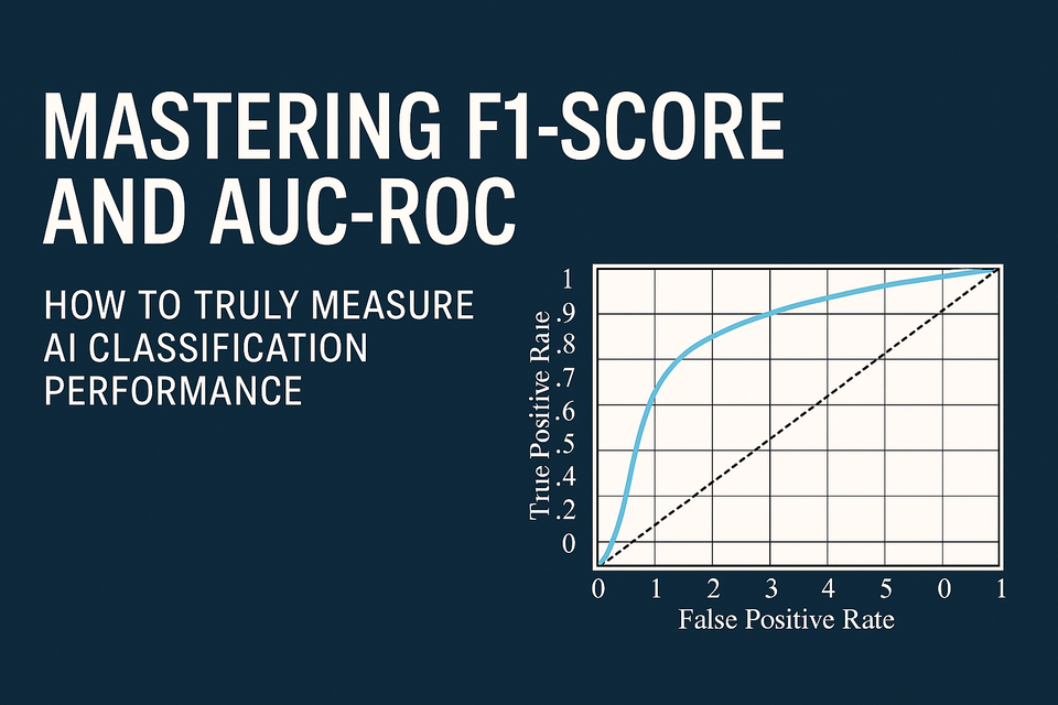
Understanding the ROC Curve

The Receiver Operating Characteristic (ROC) curve is a graphical plot that illustrates the diagnostic ability of a binary classifier system as its discrimination threshold is varied. The curve is created by plotting the True Positive Rate (TPR) against the False Positive Rate (FPR) at various threshold settings.

• True Positive Rate (TPR): This is another name for Recall (or Sensitivity). It measures the proportion of actual positives that are correctly identified as such. TPR = TP / (TP + FN)
• False Positive Rate (FPR): This measures the proportion of actual negatives that are incorrectly identified as positive. FPR = FP / (FP + TN)

To construct the ROC curve, we typically vary the classification threshold from 0.0 to 1.0 (assuming the model outputs probabilities). For each threshold:

1. We classify instances as positive or negative.
2. We calculate the TP, FP, TN, and FN counts.
3. We compute the TPR and FPR.
4. Each (FPR, TPR) pair represents a point on the ROC curve.

The ROC curve visualizes the trade-off between TPR (benefits of correctly identifying positives) and FPR (costs of incorrectly identifying negatives as positives). A model that perfectly separates the two classes would have a ROC curve that passes through the top-left corner (FPR=0, TPR=1), often referred to as the point of perfection. A model that performs no better than random guessing would have a ROC curve that is a diagonal line from (0,0) to (1,1).

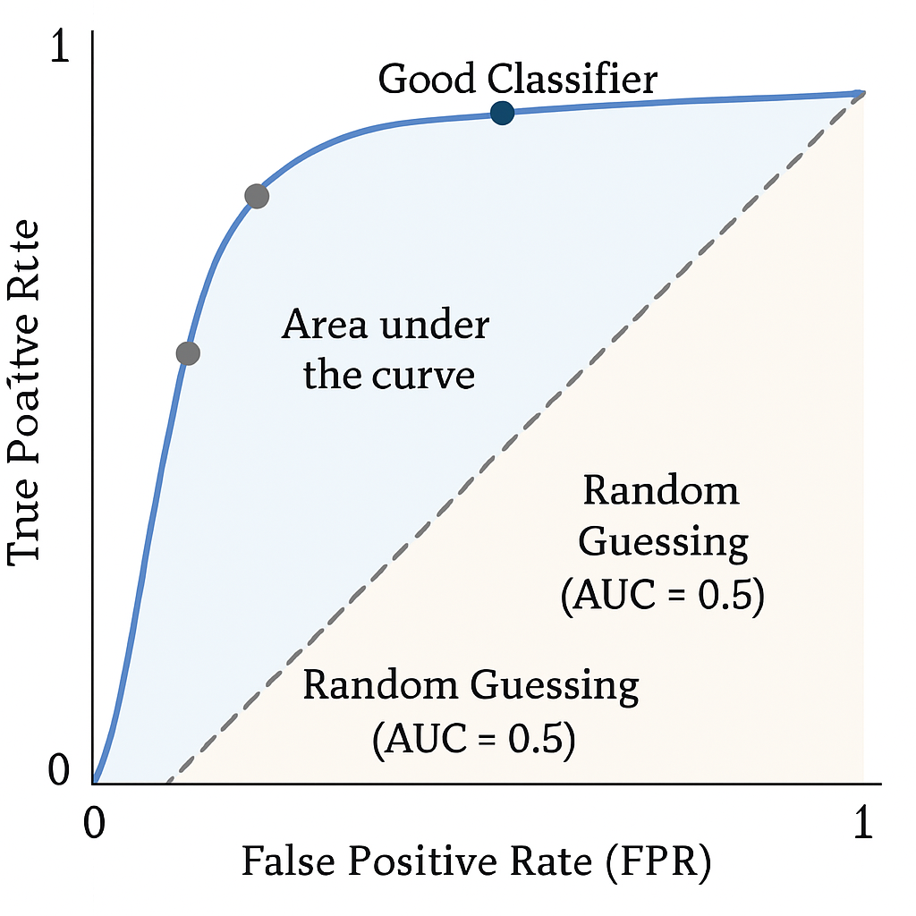
Figure 3: An example of a Receiver Operating Characteristic (ROC) curve. The blue curve represents a good classifier, with the shaded area underneath it being the AUC. The dashed diagonal line represents a random classifier (AUC = 0.5). The ideal point is the top-left corner (FPR=0, TPR=1).

The AUC: Quantifying ROC Performance

The Area Under the Curve (AUC) for the ROC curve (AUC-ROC) provides a single scalar value that summarizes the performance of the classifier across all thresholds. The AUC value ranges from 0 to 1:

• AUC = 1.0: Represents a perfect classifier. The model achieves a TPR of 1 and an FPR of 0, meaning it perfectly distinguishes between all positive and negative classes.
• AUC = 0.5: Represents a model with no discrimination ability, equivalent to random guessing (like flipping a coin). The ROC curve would be a diagonal line.
• AUC < 0.5: Represents a model that performs worse than random guessing. This often indicates that the model's predictions are inverted (e.g., it's predicting positives as negatives and vice-versa). In such cases, inverting the model's output can lead to an AUC > 0.5.
• Typically, a good model will have an AUC significantly above 0.5, with values closer to 1.0 indicating better performance.
  • 0.9–1.0: Excellent
  • 0.8–0.9: Good
  • 0.7–0.8: Fair
  • 0.6–0.7: Poor
  • 0.5–0.6: Fail

Why is AUC-ROC useful?

1. Threshold Independence: It provides a measure of how well the model can distinguish between classes, irrespective of the specific threshold chosen for classification. This is valuable when the optimal threshold is unknown or when it might change.
2. Class Separation Visualization: The ROC curve itself is a useful visualization of the model's ability to separate positive and negative instances.
3. Comparison of Models: AUC values can be directly compared to evaluate which model has better overall discrimination power.

Example: Interpreting AUC-ROC for a Spam Filter

Imagine two spam filter models:

• Model A has an AUC-ROC of 0.92.
• Model B has an AUC-ROC of 0.75.

Model A (AUC = 0.92) is significantly better at distinguishing between spam and ham emails across various probability thresholds than Model B. This means that, generally, Model A is more likely to assign higher probability scores to actual spam emails and lower scores to actual ham emails compared to Model B.

If we were to plot their ROC curves, Model A's curve would be much closer to the top-left corner of the plot than Model B's curve.

When to Prefer AUC-ROC over F1-Score?

• F1-Score is preferred when you need to choose a specific operational threshold and are concerned about the balance of precision and recall at that threshold, especially with imbalanced classes.
• AUC-ROC is preferred when you want to evaluate the model's overall ability to discriminate between classes across all possible thresholds, or when the cost of false positives and false negatives is difficult to quantify precisely for setting a single threshold.

A Note on PR-AUC (Precision-Recall AUC)

While AUC-ROC is widely used, it can sometimes be misleading for highly imbalanced datasets where the number of negative instances vastly outweighs the number of positive instances. In such scenarios, a high AUC-ROC might be achieved even if the model has poor precision for the minority (positive) class. This is because the FPR (FP / (FP + TN)) might remain low due to the large number of TNs, even with a significant number of FPs relative to TPs.

For highly imbalanced datasets, the Area Under the Precision-Recall Curve (PR-AUC or AUC-PR) is often considered a more informative metric. The Precision-Recall curve plots Precision (TP / (TP + FP)) against Recall (TPR = TP / (TP + FN)) at various thresholds.

• A perfect model would have a PR-AUC of 1.0 (Precision=1, Recall=1).
• A random baseline on a PR curve depends on the class imbalance. For a dataset with P positives and N negatives, the random baseline is P / (P+N).

PR-AUC focuses more directly on the performance on the positive (often minority) class and is less influenced by the large number of true negatives. It is particularly useful when the primary goal is to correctly identify positive instances while maintaining high precision.

In summary, AUC-ROC provides a robust, threshold-independent measure of a classifier's ability to distinguish between classes. However, for tasks with significant class imbalance where the positive class is of primary interest, complementing AUC-ROC with PR-AUC can offer a more nuanced and reliable assessment of model performance.

🧩 Final Thought

When evaluating classification models, it's rarely about a single metric. A comprehensive assessment often involves monitoring multiple indicators: F1-score (and its variants like Macro F1 and Weighted F1), Precision, Recall, the Fβ-score for tailored needs, and AUC-ROC (often complemented by PR-AUC for imbalanced datasets). Beyond these statistical measures, it's also crucial to consider business-specific Key Performance Indicators (KPIs) that reflect the real-world impact of the model's decisions.

Understanding why and when to use each metric, their strengths, their limitations, and how they interrelate, is fundamental to building effective and reliable AI systems. Choosing the right set of metrics allows you to truly understand your model's performance, identify areas for improvement, and ultimately, deploy models that achieve their intended purpose successfully. This nuanced understanding moves beyond chasing a single high score and towards developing genuinely intelligent solutions.