01 May 2025 9 min read generative-ai-news

Diving Deeper: Inside the Transformer Layer

"A clear breakdown of Transformer layers—LayerNorm, Attention, FeedForward, and Residuals—explained step-by-step with visuals."

Building upon the foundational concepts of non-linearity and activation functions discussed previously, this post delves into the core components that make up a single layer within the Transformer architecture, as introduced by Vaswani et al. (2017). Understanding these building blocks—Layer Normalization, Multi-Head Attention, FeedForward Networks, and Residual Connections—is key to grasping how Transformers process information so effectively.

The Overall Architecture

The original Transformer model consists of an encoder and a decoder, each composed of a stack of identical layers. Figure 1 from the "Attention Is All You Need" paper illustrates this overall structure:

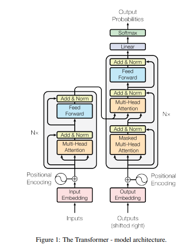
While the full encoder-decoder structure is crucial for sequence-to-sequence tasks like machine translation, many modern large language models (LLMs) primarily use the decoder stack. However, the fundamental layer structure within both is similar. We will focus on the components within one such layer.

The Flow Through a Modern Transformer Layer (Pre-LN Variant)

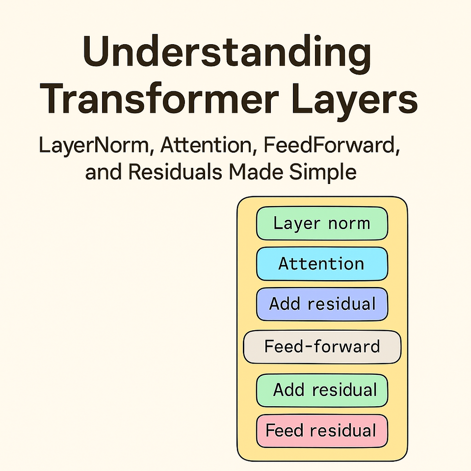
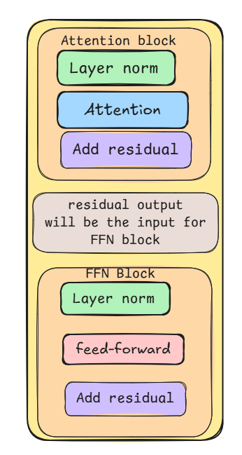
A Transformer layer processes a sequence of input vectors (embeddings), one for each token. Each vector navigates through two main sub-blocks: Multi-Head Attention and a FeedForward Network. In the widely adopted "Pre-LN" (Pre-Layer Normalization) variant, which often leads to more stable training than the original Post-LN structure (Ba et al., 2016; Xiong et al., 2020), each sub-block is preceded by Layer Normalization and followed by a Residual Connection:

Input (x)
  ↓
LayerNorm
  ↓
Multi-Head Attention
  ↓
Add Residual (x + Attention output)
  ↓
LayerNorm
  ↓
FeedForward Network
  ↓
Add Residual (previous + FFN output)
  ↓
Output → passed to next layer

Let's break down each component in more detail.

Layer Normalization: Stabilizing the Flow

Layer Normalization (LayerNorm), introduced by Ba et al. (2016), is a crucial technique for stabilizing the training of deep networks like Transformers. Unlike Batch Normalization, which normalizes across the batch dimension, LayerNorm normalizes the inputs across the features for each data sample (e.g., each token's vector) independently. This makes it highly effective for recurrent networks and Transformers where sequence lengths can vary.

The Mechanics: For a single token vector x with H hidden units (features), LayerNorm computes the mean (μ) and standard deviation (σ) across these H features:

μ = (1/H) * Σ(x_i) for i=1 to H

σ = sqrt[(1/H) * Σ(x_i - μ)^2 + ε] (ε is a small constant for numerical stability)

The normalization is then applied, followed by a learned scaling (γ) and shifting (β):

x_normalized = (x - μ) / σ

LayerNorm(x) = γ * x_normalized + β

These learnable parameters (γ and β) allow the network to adaptively control the extent of normalization, potentially learning to preserve the original representation if needed.

Why is Stabilization Necessary? An Intuitive Example: As discussed previously regarding non-linearity, deep networks can suffer from unstable training dynamics. One major cause is the differing scales of values that flow through the network. Imagine a simpler problem: predicting house prices using just two features: number of bedrooms (e.g., ranging from 1 to 5) and square footage (e.g., ranging from 500 to 5000).

Inside a neural network layer, calculations might look like: output = w1 * bedrooms + w2 * footage + bias.

Even if the number of bedrooms is a very important predictor, its small numerical range (1-5) means it contributes much less to the initial output compared to square footage (500-5000), assuming similar initial weights w1 and w2. The square footage feature "shouts louder" simply because its numbers are bigger. This can make training unstable: the network might initially focus too much on the large-scale feature, and gradients related to the smaller-scale feature might become tiny (vanish) or, in other scenarios with deep networks, updates could compound and cause values to explode.

Normalization addresses this by putting all features on a similar scale, creating a "level playing field." For instance, using z-score normalization (subtracting the mean and dividing by the standard deviation) might transform both bedroom counts and square footage values to be roughly centered around 0 with a standard deviation of 1.

Now, the calculation output = w1 * normalized_bedrooms + w2 * normalized_footage + bias is more balanced. The network can learn the true importance of each feature (w1 vs w2) based on the data patterns, not just their raw numerical scale.

In Transformers, this is even more critical. Each token is represented by a high-dimensional vector (e.g., 768 or more dimensions). As this vector passes through multiple layers of Attention and FeedForward computations, the values in different dimensions can diverge significantly. LayerNorm, applied independently to each token's vector at the start of each sub-layer (in the Pre-LN variant), ensures that the vector's components maintain a consistent scale. This prevents some dimensions from dominating calculations, stabilizes the learning process, prevents exploding/vanishing activations/gradients, and allows the model to effectively weigh the contribution of different learned features within the vector (Vaswani et al., 2017; Ba et al., 2016).

Pre-LN vs. Post-LN:

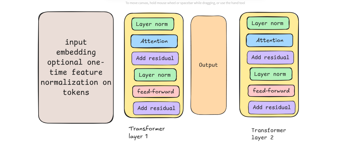
The original Transformer paper (Vaswani et al., 2017) applied LayerNorm after the residual connection (Post-LN), as shown in Figure 1 (tranformer-arch.png). However, subsequent research found that applying LayerNorm before the sub-layer and the residual connection (Pre-LN), as depicted in the layer flow diagram (layer_structure.png), often leads to more stable training dynamics and allows for training deeper models without careful initialization or learning rate warmup (Xiong et al., 2020; Nguyen & Salazar, 2019). This Pre-LN structure is now commonly used.

Residual Connections: Enabling Depth

Residual connections, also known as skip connections, were famously introduced in Residual Networks (ResNets) by He et al. (2016) to address the degradation problem encountered when training very deep neural networks. The core idea is simple yet powerful: add the input of a block directly to its output.

output = F(x) + x

Where F(x) represents the transformation performed by the block (e.g., the Attention or FFN sub-layer, potentially including LayerNorm).

Why Are They Important? As networks get deeper, gradients can struggle to propagate back through many layers during backpropagation, leading to the vanishing gradient problem and making optimization difficult. A residual connection provides a direct, unimpeded path for the gradient to flow backward. This shortcut ensures that the network can, at minimum, learn an identity mapping (where F(x) learns to output zero), meaning adding more layers is less likely to hurt performance. It encourages the network to learn only the residual—the difference or refinement F(x) that needs to be added to the input x—which is often easier than learning the entire transformation from scratch.

In Transformers: In the Transformer architecture (Vaswani et al., 2017), residual connections are applied around each of the two main sub-layers (Multi-Head Attention and FeedForward Network) within every layer. Following the Pre-LN structure:

Input to Attention: x
LayerNorm: norm_x = LayerNorm(x)
Attention: attn_output = MultiHeadAttention(norm_x)
First Residual Connection: residual1_output = x + attn_output
Input to FFN: residual1_output
LayerNorm: norm_residual1 = LayerNorm(residual1_output)
FeedForward: ffn_output = FeedForward(norm_residual1)
Second Residual Connection: layer_output = residual1_output + ffn_output

This structure ensures that the representation from the beginning of the layer (x or residual1_output) is preserved and added to the output of the complex transformations. This significantly stabilizes training, facilitates gradient flow, and allows for the construction of the very deep networks characteristic of modern LLMs.

Multi-Head Attention: Focusing on Relationships

The Multi-Head Attention mechanism, introduced by Vaswani et al. (2017), is a cornerstone of the Transformer architecture. It allows the model to jointly attend to information from different representation subspaces at different positions, effectively weighing the importance of different tokens when processing a specific token.

Scaled Dot-Product Attention: The fundamental building block is Scaled Dot-Product Attention. It operates on queries (Q), keys (K), and values (V), which are typically linear projections of the input vectors. The attention score between a query and all keys is computed using a dot product, scaled by the square root of the key dimension (dk) to prevent excessively large values. A softmax function then converts these scores into weights, which are used to compute a weighted sum of the values (Vaswani et al., 2017, Section 3.2.1).

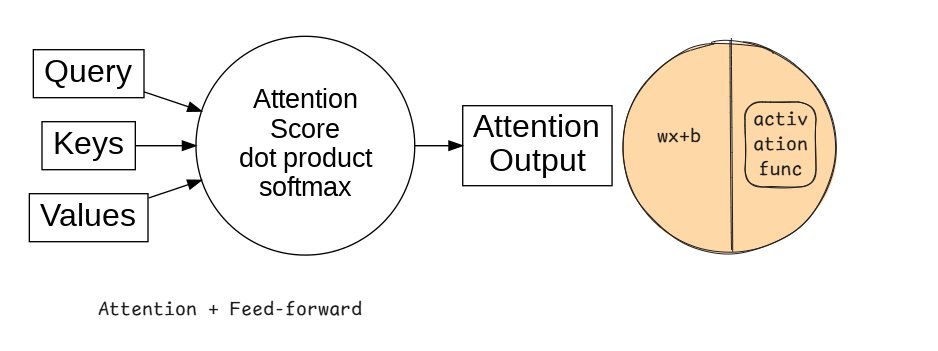
Mathematically:

Attention(Q, K, V) = softmax( (Q * K^T) / sqrt(dk) ) * V

Multi-Head Mechanism: Instead of performing a single attention function, Transformers employ "Multi-Head" Attention. The Q, K, and V vectors are linearly projected h times with different, learned linear projections. Scaled Dot-Product Attention is applied in parallel to each of these projected versions, yielding h output values. These are concatenated and once again projected linearly to produce the final output (Vaswani et al., 2017, Section 3.2.2).

MultiHead(Q, K, V) = Concat(head_1, ..., head_h) * W_o

where

head_i = Attention(Q*W_q_i, K*W_k_i, V*W_v_i)

This multi-head approach allows the model to capture different types of relationships (e.g., syntactic, semantic) in parallel, providing a richer representation compared to single-head attention.

(Note: In the encoder and the first attention block of the decoder, Q, K, and V come from the same source (the previous layer's output), referred to as self-attention. In the decoder's second attention block, Q comes from the previous decoder layer, while K and V come from the encoder's output.)

Position-wise FeedForward Networks: Adding Complexity

In addition to the attention mechanism, each layer in the Transformer contains a fully connected feed-forward network (FFN). This network is applied to each position (token) separately and identically (Vaswani et al., 2017, Section 3.3).

Structure: While the attention sub-layers handle the interaction between different positions, the FFN provides additional non-linear transformations within each position. It typically consists of two linear transformations with a non-linear activation function in between.

The most common activation function used in the original Transformer was the Rectified Linear Unit (ReLU):

FFN(x) = max(0, x*W1 + b1)*W2 + b2

Here:

x is the output from the preceding attention sub-layer (after Add & Norm).
W1 and b1 are the weights and bias of the first linear layer, which typically expands the dimensionality (e.g., from d_model to d_ff).
W2 and b2 are the weights and bias of the second linear layer, which projects the dimensionality back down (from d_ff to d_model).
The inner dimension d_ff is often significantly larger than d_model (e.g., 4 times larger in the base Transformer model).

Later models often use other activation functions like GELU (Gaussian Error Linear Unit) (Hendrycks & Gimpel, 2016) for potentially smoother gradients and improved performance.

Purpose: While the exact role is multifaceted, the FFN can be thought of as further processing the contextual information gathered by the attention mechanism. The expansion to a higher dimension (d_ff) allows the model to potentially learn more complex feature interactions before projecting back to the standard model dimension. It adds computational depth and representational capacity to each layer, complementing the sequence-mixing capabilities of the attention mechanism.

Summary: The Transformer Layer Assembled

We have dissected the core components commonly found within a single layer of modern Transformer architectures, particularly the Pre-LN variant:

Layer Normalization (Ba et al., 2016): Applied before each sub-layer, it normalizes the input across features for each token, stabilizing training.
Multi-Head Self-Attention (Vaswani et al., 2017): Allows each token to gather context by attending to other tokens in the sequence across multiple representation subspaces.
Residual Connection (He et al., 2016): Adds the input of the sub-layer to its output, facilitating gradient flow and enabling deeper networks.
Position-wise FeedForward Network (Vaswani et al., 2017): Applied independently to each token, it provides further non-linear transformations using two linear layers and an activation function (like ReLU or GELU).

The sequence within the layer typically follows: LayerNorm -> Attention -> Add Residual -> LayerNorm -> FeedForward -> Add Residual.

This modular design, repeated multiple times in stacks (as shown in Figure 1 (tranformer-arch.png) from Vaswani et al., 2017 ), forms the backbone of powerful models capable of understanding complex patterns in sequential data. While each component has further intricacies, understanding this fundamental layer structure provides a solid basis for exploring the capabilities of Transformers.

References

Vaswani, A., Shazeer, N., Parmar, N., Uszkoreit, J., Jones, L., Gomez, A. N., ... & Polosukhin, I. (2017). Attention is all you need. Advances in neural information processing systems, 30. (Available at: https://arxiv.org/abs/1706.03762)
Ba, J. L., Kiros, J. R., & Hinton, G. E. (2016). Layer normalization. arXiv preprint arXiv:1607.06450. (Available at: https://arxiv.org/abs/1607.06450)
He, K., Zhang, X., Ren, S., & Sun, J. (2016). Deep residual learning for image recognition. In Proceedings of the IEEE conference on computer vision and pattern recognition (pp. 770-778). (Available at: https://arxiv.org/abs/1512.03385)
Xiong, R., Yang, Y., He, D., Zheng, K., Zheng, S., Xing, C., ... & Liu, T. (2020). On layer normalization in the transformer architecture. In International Conference on Machine Learning (pp. 10524-10533). PMLR. (Available at: https://proceedings.mlr.press/v119/xiong20b.html or https://arxiv.org/abs/2002.04745)
Nguyen, T., & Salazar, J. (2019). Transformers without tears: Improving the normalization architecture of transformers. arXiv preprint arXiv:1910.05895. (Available at: https://arxiv.org/abs/1910.05895)
Hendrycks, D., & Gimpel, K. (2016). Gaussian Error Linear Units (GELUs). arXiv preprint arXiv:1606.08415. (Available at: https://arxiv.org/abs/1606.08415)