04 Apr 2025 37 min read GenAI

Understanding GANs: How Machines Learn to Create

“The Discriminator knows the domain. The Generator starts with nothing. It generates gibberish, gets rejected, and slowly adapts — until it produces something so good, the Discriminator can't tell anymore.”

In the rapidly evolving landscape of artificial intelligence, few innovations have captured the imagination quite like Generative Adversarial Networks, or GANs. Since their introduction by Ian Goodfellow and his colleagues in 2014, GANs have revolutionized how machines generate content, pushing the boundaries of what we thought possible in artificial creativity.

Imagine scrolling through a gallery of portraits, each face detailed and expressive, with unique features that make them appear distinctly human—only to discover that none of these people actually exist. Or consider viewing a photograph that has been transformed from a blurry, low-resolution image into a crystal-clear picture with remarkable detail. These are not science fiction scenarios but real applications of GANs in today's world.

GANs represent a paradigm shift in machine learning. Unlike traditional algorithms that learn to categorize or predict based on existing data, GANs learn to create new data that mimics the patterns and characteristics of what they've been trained on. This creative capability has led to breakthroughs across numerous domains—from generating photorealistic images and enhancing medical scans to creating synthetic data for training other AI systems and even composing music.

What makes GANs particularly fascinating is their unique learning mechanism. Rather than learning from explicit feedback about what's right or wrong, GANs learn through an adversarial process—a continuous competition between two neural networks that push each other to improve. This mimics how human artists often develop their craft through critique and refinement, making GANs one of the most "human-like" approaches to machine learning.

In this comprehensive guide, we'll demystify GANs by breaking down their inner workings, exploring their architecture, and walking through a practical implementation using the MNIST dataset of handwritten digits. The MNIST dataset serves as an ideal starting point for understanding GANs—it's simple enough to grasp the core concepts but complex enough to demonstrate the power of generative modeling.

By the end of this post, you'll understand:

The fundamental architecture of GANs and how their components interact
The mathematics behind GAN training and why it works
How to implement a basic GAN in PyTorch to generate handwritten digits
Common challenges in training GANs and strategies to overcome them
Real-world applications that have emerged from this technology

Whether you're a machine learning practitioner looking to add GANs to your toolkit, a developer curious about generative models, or simply someone fascinated by AI's creative potential, this guide will provide you with both theoretical understanding and practical knowledge to appreciate and work with this groundbreaking technology.

Let's begin our journey into the world of GANs, where mathematics meets imagination, and machines learn the art of creation.

1. What is a GAN?

At its core, a Generative Adversarial Network (GAN) represents one of the most innovative approaches to generative modeling in machine learning. Unlike traditional neural networks that learn to classify or predict, GANs learn to create new data that resembles a given dataset. What makes GANs truly unique is their architecture—a system composed of two neural networks locked in an adversarial relationship:

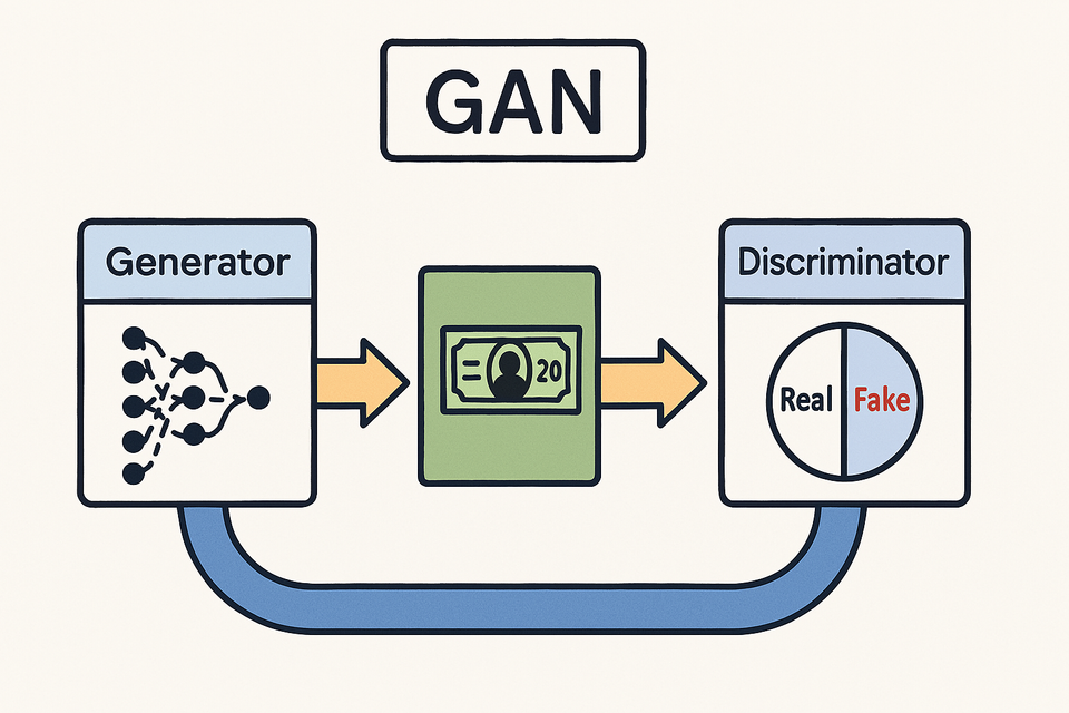
The Two Players in the GAN Game

The Generator: This neural network starts with random noise and transforms it into synthetic data (like images). Its sole purpose is to create outputs so convincing that they're indistinguishable from real data. In our MNIST implementation, the Generator takes random noise vectors and converts them into images that resemble handwritten digits.

The Discriminator: This neural network acts as a judge or critic. It receives both real data from the training set and fake data from the Generator, and its job is to correctly identify which is which. In our implementation, the Discriminator examines images and outputs a probability indicating whether it believes each image is a real MNIST digit or a Generator-created fake.

The Adversarial Relationship

The genius of GANs lies in how these networks interact. Think of the Generator as a counterfeiter trying to produce fake currency, while the Discriminator functions as a detective trying to identify the counterfeits. As the counterfeiter gets better at creating convincing fakes, the detective must become more discerning. Conversely, as the detective improves, the counterfeiter must refine their techniques to create even more convincing forgeries.

This continuous feedback loop drives both networks to improve simultaneously. The Generator never sees the real data directly—it only receives feedback through the Discriminator's judgments. This indirect learning process is what enables GANs to capture complex data distributions without explicit programming.

Looking at Our MNIST GAN Implementation

Let's examine how these concepts are implemented in our PyTorch code for generating MNIST digits:

# Generator
class Generator(nn.Module):
    def __init__(self):
        super().__init__()
        self.model = nn.Sequential(
            nn.Linear(latent_dim, 256),
            nn.ReLU(True),
            nn.Linear(256, 512),
            nn.ReLU(True),
            nn.Linear(512, 1024),
            nn.ReLU(True),
            nn.Linear(1024, 28 * 28),
            nn.Tanh()
        )

    def forward(self, z):
        out = self.model(z)
        return out.view(z.size(0), 1, 28, 28)

# Discriminator
class Discriminator(nn.Module):
    def __init__(self):
        super().__init__()
        self.model = nn.Sequential(
            nn.Linear(28 * 28, 512),
            nn.LeakyReLU(0.2, inplace=True),
            nn.Linear(512, 256),
            nn.LeakyReLU(0.2, inplace=True),
            nn.Linear(256, 1),
            nn.Sigmoid()
        )

    def forward(self, img):
        img_flat = img.view(img.size(0), -1)
        return self.model(img_flat)

Our Generator starts with a random noise vector of dimension latent_dim (set to 100 in our code). This vector passes through several fully connected layers with increasing sizes (256, 512, 1024), finally producing an output with 784 elements (28×28, the dimensions of an MNIST digit image). The Tanh activation function in the final layer ensures the output values are between -1 and 1, matching our normalized MNIST data.

The Discriminator takes an image (either real from MNIST or fake from the Generator), flattens it into a 784-element vector, and processes it through fully connected layers with decreasing sizes (512, 256), ultimately producing a single value between 0 and 1 via the Sigmoid activation function. This value represents the Discriminator's confidence that the input image is real (closer to 1) or fake (closer to 0).

Why This Architecture Works

This adversarial setup creates a minimax game where:

The Generator tries to maximize the probability that the Discriminator makes a mistake
The Discriminator tries to maximize its accuracy in distinguishing real from fake

As training progresses, both networks improve their capabilities. The Generator learns to produce increasingly realistic digits, while the Discriminator becomes more sophisticated in its ability to detect subtle differences between real and generated images. Eventually, if training is successful, the Generator will create images so convincing that the Discriminator can do no better than random guessing (a 50% chance of being correct).

This elegant competitive framework is what enables GANs to generate such impressive results across various domains, from simple handwritten digits to photorealistic human faces and beyond.

2. How GANs Work (Conceptual Flow)

Understanding the flow of data through a GAN is essential to grasping how these networks function. Let's break down the conceptual process step by step, connecting each concept to our MNIST implementation.

The GAN Data Flow

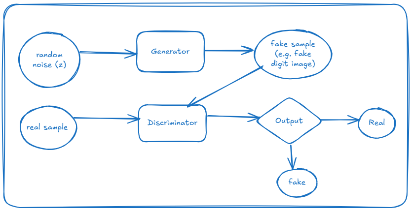
This seemingly simple diagram encapsulates the core mechanics of a GAN. Let's examine each component in detail:

1. Random Noise (Latent Space)

Every GAN generation begins with random noise, typically sampled from a normal distribution. This noise vector, often called z, serves as the seed from which the Generator creates data. In our MNIST implementation, we define this as:

latent_dim = 100
z = torch.randn(batch_size, latent_dim).to(device)

Here, torch.randn generates random numbers from a standard normal distribution (mean 0, variance 1). Each noise vector has 100 dimensions, creating a rich latent space from which our Generator can work.

The latent space is fascinating because it's not just random chaos—during training, the Generator learns to map different regions of this space to meaningful features in the output. For instance, in our digit generation task, certain dimensions might come to represent stroke thickness, digit slant, or specific shape characteristics.

2. Generator Transformation

The Generator takes this random noise and transforms it through a series of neural network layers into something that resembles our target data—in this case, handwritten digits. In our implementation:

fake_imgs = G(z)

This simple line masks the complexity happening inside the Generator. Let's revisit the Generator's architecture:

class Generator(nn.Module):
    def __init__(self):
        super().__init__()
        self.model = nn.Sequential(
            nn.Linear(latent_dim, 256),
            nn.ReLU(True),
            nn.Linear(256, 512),
            nn.ReLU(True),
            nn.Linear(512, 1024),
            nn.ReLU(True),
            nn.Linear(1024, 28 * 28),
            nn.Tanh()
        )

    def forward(self, z):
        out = self.model(z)
        return out.view(z.size(0), 1, 28, 28)

The noise vector passes through multiple fully connected layers, each followed by a ReLU activation function. The network progressively expands the representation (from 100 → 256 → 512 → 1024 → 784), ultimately reshaping the output to match the dimensions of an MNIST digit (28×28 pixels). The final Tanh activation ensures the output values are between -1 and 1, matching our normalized training data.

3. Real and Fake Samples

For training, we need both real samples from our dataset and fake samples from our Generator:

# Real samples from MNIST dataset
real_imgs = real_imgs.to(device)

# Fake samples from Generator
z = torch.randn(batch_size, latent_dim).to(device)
fake_imgs = G(z)

The real samples come directly from the MNIST dataset, which we've loaded and normalized:

transform = transforms.Compose([
    transforms.ToTensor(),
    transforms.Normalize([0.5], [0.5])  # normalize to [-1, 1]
])

train_loader = torch.utils.data.DataLoader(
    torchvision.datasets.MNIST(root='.', train=True, transform=transform, download=True),
    batch_size=batch_size,
    shuffle=True
)

4. Discriminator Evaluation

The Discriminator examines both real and fake samples, outputting a probability that each sample is real:

real_loss = loss_fn(D(real_imgs), real_labels)
fake_loss = loss_fn(D(fake_imgs.detach()), fake_labels)

Let's look at the Discriminator's architecture:

class Discriminator(nn.Module):
    def __init__(self):
        super().__init__()
        self.model = nn.Sequential(
            nn.Linear(28 * 28, 512),
            nn.LeakyReLU(0.2, inplace=True),
            nn.Linear(512, 256),
            nn.LeakyReLU(0.2, inplace=True),
            nn.Linear(256, 1),
            nn.Sigmoid()
        )

    def forward(self, img):
        img_flat = img.view(img.size(0), -1)
        return self.model(img_flat)

The Discriminator flattens the 28×28 image into a 784-element vector, processes it through fully connected layers with LeakyReLU activations, and outputs a single value between 0 and 1 via the Sigmoid function. This value represents the Discriminator's confidence that the input is a real MNIST digit.

The Information Flow During Training

What makes GANs unique is how information flows during training:

The Discriminator sees real data and learns what real MNIST digits look like.
The Generator creates fake data based on random noise.
The Discriminator evaluates the fake data and provides feedback.
The Generator uses this feedback to improve its next generation.

Crucially, the Generator never sees real data directly—it only receives feedback through the Discriminator's judgments. This indirect learning process is what enables GANs to capture complex data distributions without explicit programming.

Visualizing the Process

In our MNIST implementation, we save samples of the Generator's output at each epoch:

with torch.no_grad():
    test_z = torch.randn(64, latent_dim).to(device)
    generated = G(test_z)
    save_image(generated, f"{sample_dir}/epoch_{epoch+1:03d}.png", normalize=True, nrow=8)

These saved images create a visual timeline of the Generator's improvement. Initially, the generated digits look like random noise, but as training progresses, they gradually take on the characteristics of handwritten digits. This visual progression is one of the most intuitive ways to understand how GANs learn and improve over time.

The conceptual flow of GANs—from random noise to convincing fake samples—represents a fundamentally different approach to generative modeling. Rather than explicitly programming rules for what makes a convincing digit, we let the networks discover these patterns through their adversarial relationship, resulting in a powerful and flexible framework for generating complex data.

3. Training the GAN

Training a GAN is a delicate balancing act. Unlike traditional neural networks with a single objective function, GANs involve two networks with opposing goals. Let's break down the training process step by step, using our MNIST implementation as a practical example.

The Training Loop

At its core, GAN training alternates between updating the Discriminator and the Generator. Here's the main training loop from our MNIST implementation:

# Training loop
for epoch in range(epochs):
    for real_imgs, _ in train_loader:
        real_imgs = real_imgs.to(device)
        batch_size = real_imgs.size(0)

        # Labels
        real_labels = torch.ones(batch_size, 1).to(device)
        fake_labels = torch.zeros(batch_size, 1).to(device)

        # Train Discriminator
        z = torch.randn(batch_size, latent_dim).to(device)
        fake_imgs = G(z)
        real_loss = loss_fn(D(real_imgs), real_labels)
        fake_loss = loss_fn(D(fake_imgs.detach()), fake_labels)
        d_loss = real_loss + fake_loss

        d_optimizer.zero_grad()
        d_loss.backward()
        d_optimizer.step()

        # Train Generator
        z = torch.randn(batch_size, latent_dim).to(device)
        fake_imgs = G(z)
        g_loss = loss_fn(D(fake_imgs), real_labels)

        g_optimizer.zero_grad()
        g_loss.backward()
        g_optimizer.step()

    # Save samples
    print(f"Epoch [{epoch+1}/{epochs}]  D Loss: {d_loss.item():.4f}  G Loss: {g_loss.item():.4f}")
    with torch.no_grad():
        test_z = torch.randn(64, latent_dim).to(device)
        generated = G(test_z)
        save_image(generated, f"{sample_dir}/epoch_{epoch+1:03d}.png", normalize=True, nrow=8)

Let's break this down into detailed steps:

Step 1: Prepare Real Data and Labels

real_imgs = real_imgs.to(device)
batch_size = real_imgs.size(0)

# Labels
real_labels = torch.ones(batch_size, 1).to(device)
fake_labels = torch.zeros(batch_size, 1).to(device)

We start by moving our real MNIST images to the appropriate device (CPU or GPU). Then we create label tensors:

real_labels: Tensor of ones, representing "real" classification
fake_labels: Tensor of zeros, representing "fake" classification

These labels serve as the target values for our Binary Cross Entropy loss function.

Step 2: Train the Discriminator

# Train Discriminator
z = torch.randn(batch_size, latent_dim).to(device)
fake_imgs = G(z)
real_loss = loss_fn(D(real_imgs), real_labels)
fake_loss = loss_fn(D(fake_imgs.detach()), fake_labels)
d_loss = real_loss + fake_loss

d_optimizer.zero_grad()
d_loss.backward()
d_optimizer.step()

Training the Discriminator involves several key operations:

Generate fake images: We create random noise vectors and pass them through the Generator to produce fake MNIST digits.
Compute loss on real images: We pass real MNIST digits through the Discriminator and calculate how well it identifies them as real (ideally, D(real_imgs) should be close to 1).
Compute loss on fake images: We pass the generated fake digits through the Discriminator and calculate how well it identifies them as fake (ideally, D(fake_imgs) should be close to 0).Note the use of detach() here: fake_imgs.detach() detaches the fake images from the computation graph. This is crucial because when training the Discriminator, we want to evaluate its performance on the fake images but not update the Generator's parameters.
Combine losses: The total Discriminator loss is the sum of the real and fake losses.
Update parameters: We zero the gradients, compute the backward pass, and update the Discriminator's parameters using the optimizer.

Step 3: Train the Generator

# Train Generator
z = torch.randn(batch_size, latent_dim).to(device)
fake_imgs = G(z)
g_loss = loss_fn(D(fake_imgs), real_labels)

g_optimizer.zero_grad()
g_loss.backward()
g_optimizer.step()

Training the Generator follows a similar pattern:

Generate new fake images: We create a new batch of random noise vectors and generate fake images. Note that we generate new fake images rather than reusing those from the Discriminator training step. This provides fresh samples for the Generator to learn from.
Compute Generator loss: The Generator's goal is to fool the Discriminator, so we want the Discriminator to classify our fake images as real. Therefore, we use real_labels (all ones) as the target. The loss measures how far D(fake_imgs) is from 1.
Update parameters: We zero the gradients, compute the backward pass, and update the Generator's parameters.

Step 4: Monitor Progress and Save Samples

# Save samples
print(f"Epoch [{epoch+1}/{epochs}]  D Loss: {d_loss.item():.4f}  G Loss: {g_loss.item():.4f}")
with torch.no_grad():
    test_z = torch.randn(64, latent_dim).to(device)
    generated = G(test_z)
    save_image(generated, f"{sample_dir}/epoch_{epoch+1:03d}.png", normalize=True, nrow=8)

After each epoch (a complete pass through the training dataset), we:

Print loss values: This helps us monitor the training progress. In a healthy GAN training process, both losses should generally decrease, though they may fluctuate.
Generate and save samples: We create 64 new fake images and save them as a grid. This visual record is invaluable for tracking the Generator's improvement over time.The with torch.no_grad(): context manager tells PyTorch not to track gradients during this operation, saving memory and computation since we're just generating images for visualization, not training.

The Minimax Game

GAN training is often described as a minimax game, where:

The Discriminator tries to maximize its ability to distinguish real from fake (maximize log(D(x)) + log(1 - D(G(z))))
The Generator tries to minimize the Discriminator's ability to detect its fakes (minimize log(1 - D(G(z))))

In practice, the Generator often maximizes log(D(G(z))) instead of minimizing log(1 - D(G(z))), as this provides stronger gradients early in training.

Training Challenges

Training GANs can be notoriously difficult due to several challenges:

Balancing network strength: If the Discriminator becomes too powerful too quickly, it may provide minimal useful feedback to the Generator. Conversely, if the Generator becomes too strong, it may overwhelm the Discriminator.
Vanishing gradients: If the Discriminator confidently rejects Generator outputs, the gradients may become too small for effective learning.
Mode collapse: The Generator might learn to produce only a limited variety of outputs that fool the Discriminator, rather than capturing the full diversity of the training data.

In our MNIST implementation, we use several techniques to mitigate these issues:

Balanced architecture: Both networks have similar complexity, helping maintain balance.
Appropriate learning rates: We use a learning rate of 0.0002 for both networks.
LeakyReLU in the Discriminator: This helps prevent vanishing gradients by allowing a small gradient when the input is negative.
Regular monitoring: By saving samples at each epoch, we can detect issues like mode collapse early.

The Evolution of Generated Images

One of the most satisfying aspects of training a GAN is watching the generated images improve over time. In our MNIST implementation, the progression typically looks something like this:

Early epochs: Random noise with no discernible digit structure
Middle epochs: Blurry, digit-like shapes begin to emerge
Later epochs: Clearer digit structures with recognizable forms
Final epochs: Sharp, convincing handwritten digits

This visual progression provides intuitive confirmation that our GAN is learning effectively.

Hyperparameter Considerations

Several hyperparameters significantly impact GAN training:

Batch size: We use 128, which provides stable gradients without excessive memory usage.
Learning rate: 0.0002 is a common choice for GANs, balancing stability and training speed.
Network size: Our networks are relatively simple but sufficient for MNIST. More complex datasets would require deeper architectures.
Latent dimension: We use 100, providing ample space for the Generator to learn meaningful representations.

Training a GAN is as much an art as a science, often requiring experimentation and tuning to achieve optimal results. The process described here provides a solid foundation, but don't be afraid to adjust parameters and architectures based on your specific dataset and goals.

4. Activation Functions in GANs

Activation functions play a crucial role in neural networks, including GANs. They introduce non-linearity into the network, allowing it to learn complex patterns and relationships. In GANs, the choice of activation functions significantly impacts both the training dynamics and the quality of generated outputs.

Understanding Activation Functions

Activation functions transform the output of a neuron, determining whether and how strongly it "fires" in response to input. Let's examine the key activation functions used in GANs and why they're chosen for specific layers.

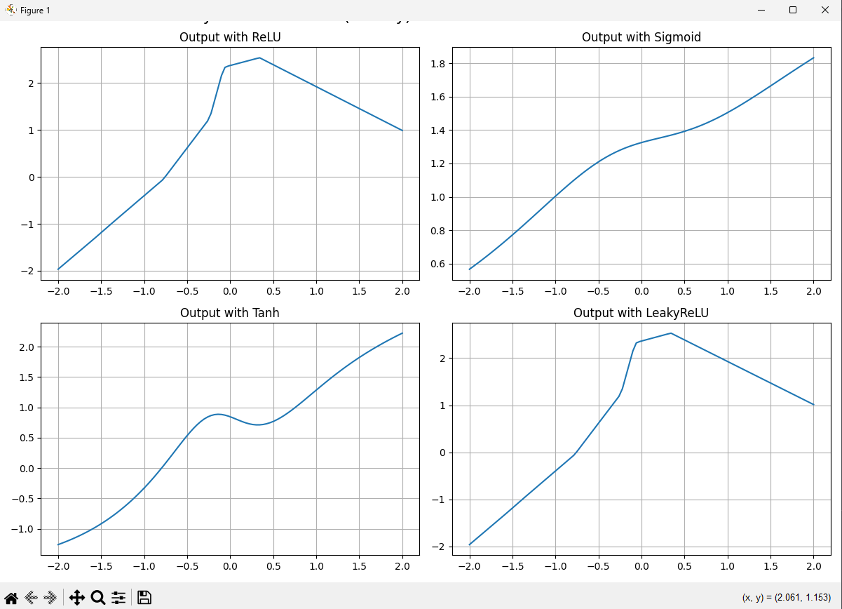
Activation Functions Comparison — Activation Functions

The image above shows how different activation functions transform inputs. Notice how each function has distinct characteristics:

ReLU (Rectified Linear Unit): Outputs the input directly if positive, otherwise outputs zero
Sigmoid: Squashes input to a range between 0 and 1
Tanh: Squashes input to a range between -1 and 1
LeakyReLU: Similar to ReLU but allows a small gradient when the input is negative

Activation Functions in the Generator

In our MNIST GAN implementation, the Generator uses the following activation functions:

class Generator(nn.Module):
    def __init__(self):
        super().__init__()
        self.model = nn.Sequential(
            nn.Linear(latent_dim, 256),
            nn.ReLU(True),
            nn.Linear(256, 512),
            nn.ReLU(True),
            nn.Linear(512, 1024),
            nn.ReLU(True),
            nn.Linear(1024, 28 * 28),
            nn.Tanh()
        )

ReLU in Hidden Layers

The Generator uses ReLU (Rectified Linear Unit) for its hidden layers. ReLU has several advantages:

Computational Efficiency: ReLU is simple to compute (max(0, x)), making it faster than more complex functions like sigmoid or tanh.
Sparsity: ReLU activations can be truly zero, leading to sparse activations and more efficient representations.
Reduced Vanishing Gradient Problem: Unlike sigmoid and tanh, ReLU doesn't saturate in the positive region, helping to mitigate the vanishing gradient problem during backpropagation.

Tanh in the Output Layer

For the final layer, the Generator uses Tanh, which squashes outputs to the range [-1, 1]. This is chosen for a specific reason:

Matching Data Normalization: Our MNIST data is normalized to the range [-1, 1], so using Tanh ensures the Generator's output matches this range exactly.
Bounded Output: Unlike ReLU (which is unbounded), Tanh provides a bounded output, which is essential for stable image generation.
Zero-Centered Output: Tanh outputs are centered around zero, which can help with the learning dynamics when the discriminator processes these outputs.

Activation Functions in the Discriminator

The Discriminator uses a different set of activation functions:

class Discriminator(nn.Module):
    def __init__(self):
        super().__init__()
        self.model = nn.Sequential(
            nn.Linear(28 * 28, 512),
            nn.LeakyReLU(0.2, inplace=True),
            nn.Linear(512, 256),
            nn.LeakyReLU(0.2, inplace=True),
            nn.Linear(256, 1),
            nn.Sigmoid()
        )

LeakyReLU in Hidden Layers

The Discriminator uses LeakyReLU for its hidden layers, with a negative slope of 0.2. LeakyReLU was chosen for specific reasons:

Preventing Dead Neurons: Unlike standard ReLU, which outputs zero for all negative inputs, LeakyReLU allows a small gradient when the input is negative (in our case, 0.2 times the input). This helps prevent "dead neurons" that might never activate and stop learning.
Improved Gradient Flow: The small slope for negative values ensures that gradients can flow even when inputs are negative, helping with the learning process.
Discriminator Stability: In GANs, the Discriminator needs to learn subtle differences between real and fake samples. LeakyReLU helps maintain gradient flow throughout the network, contributing to more stable training.

Sigmoid in the Output Layer

For the final layer, the Discriminator uses Sigmoid, which squashes outputs to the range [0, 1]:

Probability Interpretation: The Discriminator's job is to output the probability that an input is real. Sigmoid naturally maps to this [0, 1] probability range.
Binary Classification: Since the Discriminator performs binary classification (real or fake), sigmoid is the natural choice for the output activation.
Compatibility with BCE Loss: The Binary Cross Entropy loss function used in our implementation works directly with probabilities, making sigmoid the appropriate final activation.

Visualizing Activation Functions with NumPy

To better understand how these activation functions behave, let's look at a simple NumPy implementation that visualizes their effects:

import numpy as np
import matplotlib.pyplot as plt

# Define activation functions
def relu(x): return np.maximum(0, x)
def sigmoid(x): return 1 / (1 + np.exp(-x))
def tanh(x): return np.tanh(x)
def leaky_relu(x): return np.where(x > 0, x, 0.01 * x)

# Input values
X = np.linspace(-2, 2, 100).reshape(-1, 1)

# Plot results
plt.figure(figsize=(12, 8))
activations = {
    "ReLU": relu,
    "Sigmoid": sigmoid,
    "Tanh": tanh,
    "LeakyReLU": leaky_relu
}

for i, (name, fn) in enumerate(activations.items()):
    output = fn(X)
    plt.subplot(2, 2, i + 1)
    plt.plot(X, output)
    plt.title(f"Output with {name}")
    plt.grid(True)

plt.tight_layout()
plt.suptitle("Activation Functions Comparison", fontsize=16, y=1.02)
plt.show()

This code creates visualizations similar to the image shown earlier, helping us understand how each activation function transforms inputs.

The Impact of Activation Functions on GAN Performance

The choice of activation functions significantly impacts GAN performance:

Generator Output Quality: The Tanh activation in the Generator's output layer ensures that generated images have the same pixel value range as the training data, leading to more realistic outputs.
Training Stability: LeakyReLU in the Discriminator helps maintain gradient flow, preventing the "vanishing gradient" problem that can stall training.
Mode Collapse Prevention: Proper activation functions can help prevent mode collapse, where the Generator produces limited varieties of outputs.
Convergence Speed: Well-chosen activation functions can accelerate convergence by providing better gradient flow during backpropagation.

In more advanced GAN architectures, you might encounter other activation functions like ELU (Exponential Linear Unit) or SELU (Scaled Exponential Linear Unit), each with specific advantages for certain applications. However, the combination of ReLU/Tanh in the Generator and LeakyReLU/Sigmoid in the Discriminator has proven effective for many GAN implementations, including our MNIST example.

Understanding these activation functions and their roles is crucial for designing effective GANs and troubleshooting issues during training. The right activation functions can make the difference between a GAN that produces blurry, unrealistic outputs and one that generates convincing, high-quality results.

5. Loss Functions

Loss functions are the mathematical heart of GAN training, guiding both networks toward their respective goals. Understanding these functions is crucial for comprehending how GANs learn and improve over time. Let's explore the loss functions used in our MNIST GAN implementation and the mathematics behind them.

The GAN Objective Function

In the original GAN paper by Ian Goodfellow et al., the GAN objective function is formulated as a minimax game:

This formulation encapsulates the adversarial nature of GANs:

The Discriminator (D) tries to maximize this function
The Generator (G) tries to minimize it

Let's break down what this means:

Discriminator's Goal: Maximize

Implementation in PyTorch

In our MNIST implementation, we use Binary Cross Entropy (BCE) loss to approximate this objective:

# Loss and optimizers
loss_fn = nn.BCELoss()

The BCE loss is defined as:

Where:

y is the target (0 for fake, 1 for real)
y^ is the predicted probability
N is the number of samples

Discriminator Loss

In our implementation, the Discriminator loss is calculated as:

real_loss = loss_fn(D(real_imgs), real_labels)
fake_loss = loss_fn(D(fake_imgs.detach()), fake_labels)
d_loss = real_loss + fake_loss

Breaking this down:

Real Loss: BCE(D(real_imgs),real_labels)
- This measures how well the Discriminator identifies real images.
- real_labels are all ones, so this simplifies to -log(D(real_imgs))
- The Discriminator aims to maximize D(real_imgs), making this term approach zero.
Fake Loss: BCE(D(fake_imgs),fake_labels)
- This measures how well the Discriminator identifies fake images.
- fake_labels are all zeros, so this simplifies to −log(1−D(fake_imgs))
- The Discriminator aims to minimize D(fake_imgs), making this term approach zero.
Total Loss: The sum of real and fake losses.
- The Discriminator aims to minimize this total loss.

Generator Loss

The Generator loss is calculated as:

g_loss = loss_fn(D(fake_imgs), real_labels)

This is BCE(D(fake_imgs),real_labels), which measures how well the Generator fools the Discriminator.

Since real_labels are all ones, this simplifies to -log(D(fake_imgs)). The Generator aims to maximize D(fake_imgs), making this term approach zero.

Non-Saturating Generator Loss

In practice, the original GAN formulation can lead to vanishing gradients for the Generator, especially early in training when the Discriminator can easily distinguish real from fake samples. To address this, we often use a non-saturating version of the Generator loss:

Instead of minimizing log(1 - D(G(z))), we maximize log(D(G(z))).

This is exactly what our implementation does:

g_loss = loss_fn(D(fake_imgs), real_labels)

This provides stronger gradients early in training, helping the Generator learn more effectively.

Loss Dynamics During Training

During training, we expect to see specific patterns in the loss values:

Early Training:
- Discriminator loss decreases rapidly as it learns to distinguish the initially poor Generator outputs.
- Generator loss may increase initially as the Discriminator gets better.
Mid Training:
- Both losses should stabilize somewhat, with the Discriminator maintaining a slight edge.
- Generator outputs begin to resemble the target distribution.
Late Training:
- In an ideal scenario, both losses converge to similar values.
- When the Generator perfectly captures the data distribution, the Discriminator can do no better than random guessing (0.5 probability), resulting in a theoretical equilibrium where both losses approach log(0.5) approx.~ 0.693.

Practical Considerations

Several practical considerations affect how these loss functions behave:

Label Smoothing: Instead of using hard targets (0 and 1), some implementations use smoothed labels (e.g., 0.1 and 0.9) to prevent the Discriminator from becoming too confident.
One-Sided Label Smoothing: Only smoothing the real labels (e.g., 0.9 instead of 1.0) can help prevent the Discriminator from providing overly confident feedback.
Alternative Loss Functions: More advanced GANs may use different loss functions, such as Wasserstein loss (WGAN), which can provide more stable training.
Gradient Penalties: Some implementations add gradient penalty terms to the loss function to enforce Lipschitz constraints on the Discriminator, improving stability.

Our MNIST implementation uses the standard BCE loss without these modifications, which is sufficient for this relatively simple task. However, for more complex datasets or architectures, these modifications can be crucial for successful training.

Understanding the mathematics behind GAN loss functions provides insight into the training dynamics and can help diagnose and address issues that arise during training. The adversarial nature of these loss functions—each network trying to optimize its own objective at the expense of the other—is what drives the remarkable generative capabilities of GANs.

6. Code Walkthrough (Simplified GAN in PyTorch)

Now that we've covered the theoretical aspects of GANs, let's dive into a detailed walkthrough of our MNIST GAN implementation. This section will break down the code piece by piece, explaining the purpose and functionality of each component.

Setting Up the Environment

We begin by importing the necessary libraries and defining our configuration parameters:

import torch
import torch.nn as nn
import torch.optim as optim
import torchvision
import torchvision.transforms as transforms
from torchvision.utils import save_image, make_grid
import os

# Settings
latent_dim = 100
epochs = 50
batch_size = 128
sample_dir = 'gan_samples'

os.makedirs(sample_dir, exist_ok=True)

Let's examine these components:

PyTorch Libraries: We import core PyTorch modules for neural networks (nn), optimization (optim), and vision-related utilities (torchvision).
Configuration Parameters:
- latent_dim = 100: The dimensionality of our random noise vector input to the Generator.
- epochs = 50: The number of complete passes through the training dataset.
- batch_size = 128: The number of samples processed in each training iteration.
- sample_dir = 'gan_samples': The directory where generated images will be saved.
Directory Creation: os.makedirs(sample_dir, exist_ok=True) ensures the output directory exists, creating it if necessary.

Data Preparation

Next, we prepare the MNIST dataset:

# Data Loader
transform = transforms.Compose([
    transforms.ToTensor(),
    transforms.Normalize([0.5], [0.5])  # normalize to [-1, 1]
])

train_loader = torch.utils.data.DataLoader(
    torchvision.datasets.MNIST(root='.', train=True, transform=transform, download=True),
    batch_size=batch_size,
    shuffle=True
)

This code:

Defines Transformations:
- transforms.ToTensor(): Converts PIL images to PyTorch tensors.
- transforms.Normalize([0.5], [0.5]): Normalizes pixel values from [0, 1] to [-1, 1]. This is crucial because our Generator's output layer uses Tanh, which produces values in the range [-1, 1].
Creates a DataLoader:
- Downloads the MNIST dataset if not already present.
- Applies the defined transformations.
- Sets the batch size and enables shuffling for randomized training.

Network Architectures

Now let's examine our Generator and Discriminator architectures:

Generator

# Generator
class Generator(nn.Module):
    def __init__(self):
        super().__init__()
        self.model = nn.Sequential(
            nn.Linear(latent_dim, 256),
            nn.ReLU(True),
            nn.Linear(256, 512),
            nn.ReLU(True),
            nn.Linear(512, 1024),
            nn.ReLU(True),
            nn.Linear(1024, 28 * 28),
            nn.Tanh()
        )

    def forward(self, z):
        out = self.model(z)
        return out.view(z.size(0), 1, 28, 28)

The Generator:

Takes random noise as input: A vector of size latent_dim (100).
Processes through fully connected layers: The network progressively expands the representation (100 → 256 → 512 → 1024 → 784).
Uses ReLU activations in hidden layers for non-linearity.
Uses Tanh activation in the output layer to ensure values are in the range [-1, 1].
Reshapes the output to match MNIST image dimensions (28×28 pixels).

Discriminator

# Discriminator
class Discriminator(nn.Module):
    def __init__(self):
        super().__init__()
        self.model = nn.Sequential(
            nn.Linear(28 * 28, 512),
            nn.LeakyReLU(0.2, inplace=True),
            nn.Linear(512, 256),
            nn.LeakyReLU(0.2, inplace=True),
            nn.Linear(256, 1),
            nn.Sigmoid()
        )

    def forward(self, img):
        img_flat = img.view(img.size(0), -1)
        return self.model(img_flat)

The Discriminator:

Takes an image as input: Either a real MNIST digit or a Generator-created fake.
Flattens the image from 28×28 to a 784-element vector.
Processes through fully connected layers: The network progressively reduces the representation (784 → 512 → 256 → 1).
Uses LeakyReLU activations in hidden layers with a negative slope of 0.2 to prevent dead neurons.
Uses Sigmoid activation in the output layer to produce a probability between 0 and 1.

Model Initialization

After defining our architectures, we initialize the models and prepare for training:

# Initialize models
G = Generator()
D = Discriminator()
device = torch.device('cuda' if torch.cuda.is_available() else 'cpu')
G.to(device)
D.to(device)

# Loss and optimizers
loss_fn = nn.BCELoss()
g_optimizer = optim.Adam(G.parameters(), lr=0.0002)
d_optimizer = optim.Adam(D.parameters(), lr=0.0002)

This code:

Creates instances of our Generator and Discriminator.
Determines the device (GPU if available, otherwise CPU).
Moves models to the appropriate device.
Sets up Binary Cross Entropy loss for both networks.
Configures Adam optimizers with a learning rate of 0.0002, which is a common choice for GANs.

Training Loop

The heart of our implementation is the training loop:

# Training loop
for epoch in range(epochs):
    for real_imgs, _ in train_loader:
        real_imgs = real_imgs.to(device)
        batch_size = real_imgs.size(0)

        # Labels
        real_labels = torch.ones(batch_size, 1).to(device)
        fake_labels = torch.zeros(batch_size, 1).to(device)

        # Train Discriminator
        z = torch.randn(batch_size, latent_dim).to(device)
        fake_imgs = G(z)
        real_loss = loss_fn(D(real_imgs), real_labels)
        fake_loss = loss_fn(D(fake_imgs.detach()), fake_labels)
        d_loss = real_loss + fake_loss

        d_optimizer.zero_grad()
        d_loss.backward()
        d_optimizer.step()

        # Train Generator
        z = torch.randn(batch_size, latent_dim).to(device)
        fake_imgs = G(z)
        g_loss = loss_fn(D(fake_imgs), real_labels)

        g_optimizer.zero_grad()
        g_loss.backward()
        g_optimizer.step()

    # Save samples
    print(f"Epoch [{epoch+1}/{epochs}]  D Loss: {d_loss.item():.4f}  G Loss: {g_loss.item():.4f}")
    with torch.no_grad():
        test_z = torch.randn(64, latent_dim).to(device)
        generated = G(test_z)
        save_image(generated, f"{sample_dir}/epoch_{epoch+1:03d}.png", normalize=True, nrow=8)

Let's break down this complex loop:

Outer Loop (Epochs)

The outer loop iterates through each epoch (complete pass through the dataset).

Inner Loop (Batches)

The inner loop processes each batch of real images from the MNIST dataset.

Discriminator Training

Prepare labels: Create tensors of ones for real images and zeros for fake images.
Generate fake images: Create random noise and pass it through the Generator.
Compute Discriminator loss: Calculate loss for both real and fake images.
Update Discriminator: Zero gradients, compute backward pass, and update parameters.

Note the use of fake_imgs.detach() when computing the Discriminator's loss on fake images. This detaches the fake images from the computation graph, ensuring that only the Discriminator's parameters are updated during this step.

Generator Training

Generate new fake images: Create fresh random noise and generate new fake images.
Compute Generator loss: Calculate how well these fake images fool the Discriminator.
Update Generator: Zero gradients, compute backward pass, and update parameters.

Monitoring and Visualization

After each epoch:

Print loss values: Display the current Discriminator and Generator losses.
Generate and save samples: Create 64 new fake images and save them as a grid.

The with torch.no_grad(): context ensures that no gradients are computed during this visualization step, saving memory and computation.

Visualizing the Results

The training loop saves generated images at each epoch, allowing us to visualize the Generator's progress:

with torch.no_grad():
    test_z = torch.randn(64, latent_dim).to(device)
    generated = G(test_z)
    save_image(generated, f"{sample_dir}/epoch_{epoch+1:03d}.png", normalize=True, nrow=8)

This code:

Creates random noise vectors: 64 vectors of dimension latent_dim.
Generates fake images: Passes the noise through the Generator.
Saves the images: Creates a grid of 8×8 images and saves it with the epoch number in the filename.

The normalize=True parameter ensures the images are properly scaled for visualization, and nrow=8 arranges the 64 images in a grid with 8 columns.

Code Design Considerations

Several design choices in our implementation are worth highlighting:

Simplicity: We use a straightforward architecture with fully connected layers rather than convolutional layers. While convolutional architectures (DCGANs) often perform better for image generation, this simpler approach is easier to understand and still works well for MNIST.
Balanced Architecture: The Generator and Discriminator have similar complexity, helping maintain balance during training.
Hyperparameter Choices:
- Learning rate of 0.0002 is a common choice for GANs.
- Batch size of 128 provides stable gradients without excessive memory usage.
- 50 epochs is sufficient for MNIST but might need adjustment for more complex datasets.
Regular Monitoring: Saving samples at each epoch allows us to track the Generator's progress visually.

This implementation provides a solid foundation for understanding GANs. For more complex datasets or applications, you might need to explore more sophisticated architectures like DCGANs (Deep Convolutional GANs), WGANs (Wasserstein GANs), or conditional GANs, but the core principles remain the same.

7. Visualizing GAN Training

One of the most fascinating aspects of GAN training is watching the Generator's output evolve over time. In this section, we'll explore how to visualize this progression and interpret what we're seeing.

The Evolution of Generated Images

When training a GAN on the MNIST dataset, we can observe a remarkable transformation in the Generator's output:

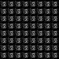
This animation shows how the Generator's output evolves across training epochs. Let's analyze what's happening at each stage:

Initial Epochs: The Generator produces random noise with no discernible structure. At this point, the Generator has not yet learned meaningful patterns from the MNIST dataset.
Early Progress: Vague digit-like shapes begin to emerge from the noise. The Generator is starting to capture the basic structure of handwritten digits, though the outputs remain blurry and indistinct.
Mid-Training: The shapes become more recognizable as digits. Different digit classes (0-9) begin to appear across the generated samples, showing that the Generator is learning the diversity of the dataset.
Later Epochs: The digits become sharper and more defined. The Generator has learned to produce convincing handwritten digits that closely resemble those in the MNIST dataset.

This visual progression provides intuitive confirmation that our GAN is learning effectively. In our implementation, we save these visual snapshots at each epoch:

# Save samples
with torch.no_grad():
    test_z = torch.randn(64, latent_dim).to(device)
    generated = G(test_z)
    save_image(generated, f"{sample_dir}/epoch_{epoch+1:03d}.png", normalize=True, nrow=8)

Creating the Animation

The GIF animation shown above can be created from the saved epoch images using tools like imageio in Python:

import imageio
import glob

# Create a GIF from saved images
images = []
for filename in sorted(glob.glob(f"{sample_dir}/epoch_*.png")):
    images.append(imageio.imread(filename))
    
imageio.mimsave('gan_training.gif', images, fps=5)

This code:

Collects all the saved epoch images in order
Reads each image into memory
Combines them into a GIF animation with 5 frames per second

Tracking Loss Values

While visual inspection is valuable, tracking loss values provides a more quantitative view of training progress:

# Assuming we've stored loss values during training
plt.figure(figsize=(10, 5))
plt.plot(d_losses, label='Discriminator Loss')
plt.plot(g_losses, label='Generator Loss')
plt.xlabel('Epoch')
plt.ylabel('Loss')
plt.legend()
plt.grid(True)
plt.title('GAN Training Loss')
plt.savefig('loss_curve.png')
plt.close()

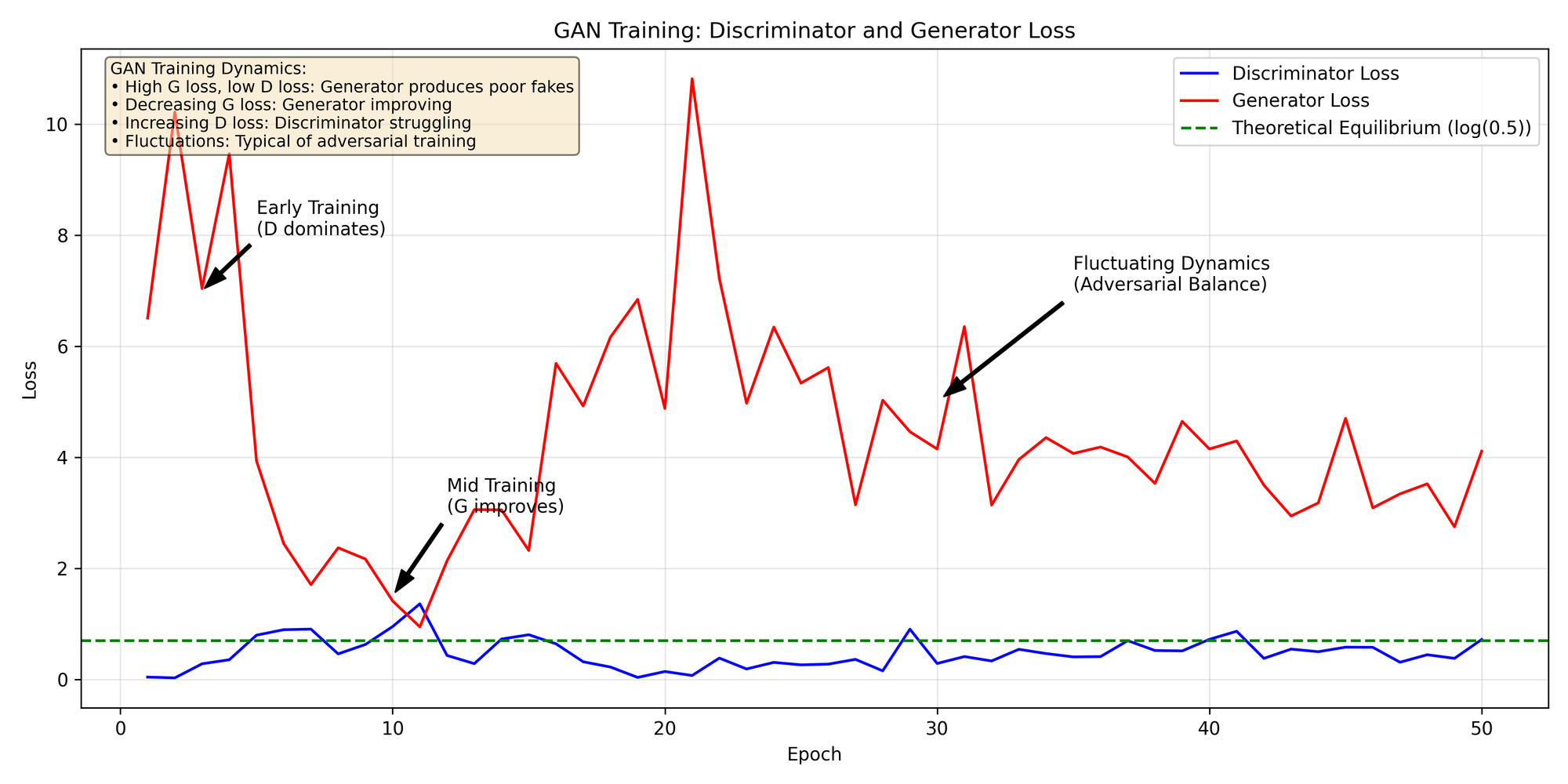
A typical loss curve for GAN training might show:

Initial Fluctuation: Both losses may be volatile at first as the networks adjust.
Discriminator Dominance: The Discriminator often learns faster initially, resulting in a lower loss.

Convergence: In successful training, both losses should eventually stabilize, though they may never completely converge to a single value.
Here is the GAN loss curve for the sample we used:

Interpreting Visual Results

When examining generated MNIST digits, look for these quality indicators:

Diversity: A good Generator should produce all digit classes (0-9), not just a few. Limited variety suggests mode collapse.
Sharpness: The digits should have clear, defined edges similar to the real MNIST digits.
Consistency: While each digit should be unique, they should all maintain the characteristic style of MNIST handwriting.
Realism: The generated digits should be difficult to distinguish from real MNIST digits.

The Latent Space

Another fascinating visualization is exploring the latent space of the Generator. By interpolating between different random noise vectors, we can see how the Generator transitions between different digit forms:

# Generate interpolation between two random points in latent space
z1 = torch.randn(1, latent_dim).to(device)
z2 = torch.randn(1, latent_dim).to(device)

n_steps = 10
samples = []

with torch.no_grad():
    for i in range(n_steps + 1):
        # Linear interpolation
        alpha = i / n_steps
        z = z1 * (1 - alpha) + z2 * alpha
        sample = G(z)
        samples.append(sample)
    
    # Concatenate and save
    samples = torch.cat(samples, 0)
    save_image(samples, "interpolation.png", normalize=True, nrow=n_steps+1)

This interpolation can reveal whether the Generator has learned a smooth, continuous representation of the digit space, or if there are abrupt transitions that indicate gaps in its understanding.

Comparing Real vs. Generated Samples

A side-by-side comparison of real and generated samples provides a clear assessment of the Generator's performance:

# Get a batch of real samples
real_batch, _ = next(iter(train_loader))
real_batch = real_batch[:32]  # Take first 32 samples

# Generate fake samples
with torch.no_grad():
    z = torch.randn(32, latent_dim).to(device)
    fake_batch = G(z)

# Concatenate real and fake samples
comparison = torch.cat([real_batch, fake_batch.cpu()], 0)
save_image(comparison, "real_vs_fake.png", normalize=True, nrow=8)

In this comparison:

The top rows show real MNIST digits
The bottom rows show generated digits

The closer these appear in style, clarity, and diversity, the better our Generator is performing.

Beyond MNIST: Visualizing Complex GANs

While MNIST provides a clear, interpretable case for visualization, these techniques extend to more complex datasets:

Face Generation: With models like StyleGAN, we can visualize the progression from noise to photorealistic human faces.
Image-to-Image Translation: For models like Pix2Pix or CycleGAN, we can show side-by-side comparisons of input images, target images, and generated outputs.
High-Resolution Generation: For models generating high-resolution images, we can zoom in on specific regions to examine fine details and textures.

Visualization is not just a way to showcase results—it's an essential tool for diagnosing issues, tracking progress, and understanding what our GAN has learned. The visual nature of GANs makes them particularly well-suited to this kind of analysis, providing insights that might be difficult to obtain from numerical metrics alone.

8. Challenges in Training GANs

While GANs are powerful generative models, they are notoriously difficult to train. Understanding these challenges is crucial for successfully implementing GANs in practice. Let's explore the common issues that arise during GAN training and strategies to address them.

Mode Collapse

Problem: Mode collapse occurs when the Generator produces only a limited variety of outputs, failing to capture the full diversity of the training data. In extreme cases, it might generate only a single type of output that reliably fools the Discriminator.

Example: In our MNIST implementation, mode collapse would manifest as the Generator producing only a few digit types (e.g., only generating variations of "1" and "7") instead of the full range of digits from 0-9.

Causes:

The Generator finds a "sweet spot" that consistently fools the Discriminator
The Discriminator provides insufficient gradient information for the Generator to learn the full data distribution
Training dynamics that allow the Generator to optimize for a local minimum rather than exploring the full space

Solutions:

Minibatch Discrimination: Allow the Discriminator to look at multiple samples together, helping it detect lack of variety
Feature Matching: Force the Generator to match the statistics of features in intermediate layers of the Discriminator
Wasserstein Loss: Use Wasserstein distance (WGAN) instead of Jensen-Shannon divergence to provide more stable gradients
Unrolled GANs: Update the Generator using gradients from multiple future Discriminator steps

In our MNIST implementation, we can detect mode collapse by examining the variety of digits in our saved sample images. If we notice limited diversity, we might need to adjust our architecture or training approach.

Non-Convergence

Problem: GANs may fail to converge to a stable equilibrium, with the loss values for both networks oscillating wildly or diverging instead of stabilizing.

Causes:

The adversarial nature creates a moving target for both networks
Imbalance between Generator and Discriminator capabilities
Poor choice of hyperparameters (learning rate, batch size, etc.)
Architectural issues that make optimization difficult

Solutions:

Balanced Architecture: Ensure neither network is significantly more powerful than the other
Learning Rate Scheduling: Gradually reduce learning rates during training
Gradient Penalty: Add a penalty term to enforce Lipschitz constraint on the Discriminator (as in WGAN-GP)
Spectral Normalization: Normalize the weights in the Discriminator to control its Lipschitz constant
Two Time-Scale Update Rule (TTUR): Use different learning rates for the Generator and Discriminator

In our implementation, we use the same learning rate (0.0002) for both networks, which works well for MNIST but might need adjustment for more complex datasets.

Vanishing Gradients

Problem: If the Discriminator becomes too confident in its predictions (outputs very close to 0 or 1), the gradients can become extremely small, providing minimal useful feedback to the Generator.

Causes:

Discriminator learns too quickly compared to the Generator
Sigmoid activation in the Discriminator output layer saturates
Poor initialization leading to extreme activation values

Solutions:

Label Smoothing: Use soft labels (e.g., 0.9 instead of 1.0 for real samples) to prevent the Discriminator from becoming too confident
LeakyReLU: Use LeakyReLU instead of ReLU in the Discriminator to allow gradient flow for negative inputs
Alternative Loss Functions: Use loss functions that provide non-vanishing gradients, such as Wasserstein loss
Batch Normalization: Apply batch normalization to stabilize activations

Our MNIST implementation already incorporates LeakyReLU in the Discriminator, which helps address this issue.

Training Instability

Problem: GAN training can be highly unstable, with performance suddenly deteriorating after periods of apparent progress.

Causes:

The adversarial nature creates a non-stationary learning problem
Small changes in either network can dramatically affect the other
Sensitivity to hyperparameter choices and initialization

Solutions:

Gradient Clipping: Limit the magnitude of gradients to prevent extreme updates
Historical Averaging: Include a term in the cost function that penalizes parameter values that deviate significantly from their historical average
Experience Replay: Keep a buffer of generated samples from previous iterations and train the Discriminator on a mix of current and past samples
Progressive Growing: Start with low-resolution images and gradually increase resolution during training (for image GANs)

Evaluation Challenges

Problem: Unlike supervised learning models, GANs lack a single, clear metric for evaluation, making it difficult to determine when training should stop or which model is "best."

Solutions:

Inception Score (IS): Measures both the quality and diversity of generated images
Fréchet Inception Distance (FID): Compares the statistics of generated images to real images
Visual Inspection: Regularly examine generated samples for quality and diversity
User Studies: For some applications, human evaluation of the generated content is the most relevant metric

In our MNIST implementation, we rely primarily on visual inspection of the generated samples, which is sufficient for this relatively simple dataset.

Practical Tips for Training GANs

Based on these challenges, here are some practical tips for training GANs:

Start Simple: Begin with a simpler architecture and dataset before tackling more complex problems.
Monitor Closely: Save generated samples frequently and watch for signs of mode collapse or training instability.
Balance is Key: Ensure neither network consistently outperforms the other. If the Discriminator becomes too powerful, the Generator may never learn effectively.
Patience and Experimentation: GAN training often requires patience and experimentation with different hyperparameters and architectural choices.
Use Established Techniques: When possible, incorporate proven techniques like batch normalization, spectral normalization, or Wasserstein loss.
Ensemble Approach: Consider training multiple GANs with different initializations and creating an ensemble of Generators.

Despite these challenges, the results of successful GAN training can be remarkable. The field continues to evolve rapidly, with new techniques and architectures regularly emerging to address these issues and push the boundaries of what GANs can achieve.

9. Real-World Applications

While our MNIST example provides an excellent introduction to GANs, the real power of this technology becomes apparent when we look at its diverse applications across various domains. Let's explore some of the most impressive and impactful real-world applications of GANs.

Image Generation and Manipulation

This Person Does Not Exist (StyleGAN)

One of the most striking demonstrations of GAN capabilities is the website "This Person Does Not Exist," which uses StyleGAN to generate photorealistic human faces that don't belong to any real person. StyleGAN, developed by NVIDIA researchers, represents a significant advancement in GAN architecture:

Progressive Growing: Training begins with low-resolution images and gradually increases resolution
Style-based Generator: Separates high-level attributes (pose, face shape) from stochastic variation (freckles, hair)
Adaptive Instance Normalization: Allows better control over the generated image style

The results are so convincing that most people cannot distinguish these AI-generated faces from photographs of real people. This technology has implications for privacy, digital content creation, and even ethical considerations around synthetic media.

Image-to-Image Translation

GANs excel at translating images from one domain to another while preserving structural content. Two notable implementations are:

Pix2Pix: A conditional GAN that learns mappings between paired images, such as:

Sketches to colored images
Black and white photos to color
Aerial photos to maps
Day scenes to night scenes

CycleGAN: Extends this concept to unpaired image translation through cycle consistency loss, enabling transformations like:

Horses to zebras
Summer to winter landscapes
Monet paintings to photographs
Apples to oranges

These technologies have applications in art, design, architecture visualization, and content creation.

Super Resolution (SRGAN)

Super Resolution GANs can upscale low-resolution images to higher resolutions while adding realistic details:

4x Upscaling: Commonly used to increase resolution by a factor of 4
Perceptual Loss: Focuses on generating visually pleasing results rather than pixel-perfect reconstructions
Adversarial Training: Helps generate high-frequency details that make images look sharp

This technology is valuable for:

Enhancing old photographs and videos
Improving medical imaging
Satellite imagery analysis
Restoring damaged visual content

Text and Language Applications

Text-to-Image Synthesis

Models like DALL-E, Midjourney, and Stable Diffusion combine GANs with other techniques to generate images from text descriptions:

Multimodal Learning: Bridging the gap between textual descriptions and visual representations
Controllable Generation: Creating specific visual content based on detailed text prompts
Creative Assistance: Helping artists and designers visualize concepts quickly

These systems can generate everything from photorealistic scenes to artistic interpretations based on text prompts.

Text Generation and Style Transfer

GANs can also be applied to text generation and style transfer:

TextGAN: Generating coherent paragraphs of text
Style Transfer: Rewriting text in different styles (formal to casual, technical to simple)
Content Generation: Creating marketing copy, product descriptions, or creative writing

Audio and Music

Voice Conversion and Synthesis

GANs have revolutionized voice technology:

Voice Conversion: Transforming one person's voice to sound like another
Text-to-Speech: Generating natural-sounding speech from text
Voice Restoration: Enhancing poor quality audio recordings

Music Generation

GANs can compose and generate music:

MuseGAN: Creating multi-track music with harmonious instruments
TimbreTron: Transferring musical style between instruments
Accompaniment Generation: Creating backing tracks for solo performances

Data Augmentation and Privacy

Data Augmentation

GANs provide a powerful tool for data augmentation in domains where data is scarce:

Medical Imaging: Generating synthetic medical images to train diagnostic systems
Rare Event Simulation: Creating examples of rare scenarios for training safety systems
Balanced Datasets: Generating additional samples for underrepresented classes

This application is particularly valuable in fields like healthcare, where privacy concerns and rare conditions limit data availability.

Differential Privacy

GANs can help protect privacy while still enabling useful data analysis:

Synthetic Data Generation: Creating realistic but non-real patient records for research
Privacy-Preserving Data Sharing: Enabling collaboration without exposing sensitive information
Anonymization: Generating modified versions of data that preserve statistical properties but protect individual privacy

Scientific Applications

Drug Discovery

GANs are accelerating pharmaceutical research:

Molecule Generation: Designing new molecular structures with desired properties
Drug Repurposing: Identifying existing drugs that might be effective for new conditions
Protein Folding: Predicting protein structures from amino acid sequences

Physics Simulations

GANs can speed up complex simulations:

Fluid Dynamics: Generating realistic fluid simulations faster than traditional methods
Particle Physics: Simulating particle interactions for high-energy physics research
Climate Modeling: Creating detailed climate predictions with less computational resources

From MNIST to State-of-the-Art

The principles we've explored in our MNIST implementation form the foundation for these advanced applications. The progression from generating simple handwritten digits to creating photorealistic human faces illustrates the remarkable scalability of GAN concepts:

Basic Principles Remain: The adversarial relationship between Generator and Discriminator remains central
Architectural Evolution: More complex datasets require more sophisticated architectures (convolutional layers, attention mechanisms)
Specialized Loss Functions: Advanced applications often use custom loss functions beyond simple BCE
Conditional Inputs: Many practical applications use conditional GANs that accept additional input to guide generation

Ethical Considerations

The power of GANs also raises important ethical considerations:

Deepfakes: GANs can create convincing fake videos, raising concerns about misinformation
Identity Theft: Generated faces could be used to create fake profiles or identities
Copyright Issues: When GANs are trained on copyrighted material, the legal status of their outputs remains unclear
Bias Amplification: GANs can amplify biases present in training data

Responsible development and deployment of GAN technology requires addressing these concerns through technical safeguards, policy frameworks, and public education.

The Future of GANs

As GAN technology continues to evolve, we can expect:

Multimodal GANs: Systems that work across multiple types of data (text, image, audio)
Interactive Generation: More intuitive interfaces for controlling GAN outputs
Efficiency Improvements: Faster training and generation with less computational resources
Specialized Architectures: GANs tailored to specific industries and applications

The journey from our simple MNIST GAN to these advanced applications demonstrates the remarkable versatility and potential of generative adversarial networks. As you continue to explore GANs, remember that the fundamental concepts we've covered provide the foundation for understanding even the most sophisticated implementations.

10. Final Thoughts

Generative Adversarial Networks represent one of the most fascinating intersections of mathematics, computer science, and creativity in modern artificial intelligence. Throughout this blog post, we've journeyed from the fundamental concepts of GANs to their practical implementation and real-world applications.

The Power of Adversarial Learning

What makes GANs truly remarkable is their unique learning mechanism. Unlike traditional supervised learning approaches that rely on explicit labels, GANs learn through competition. This adversarial process—the Generator constantly trying to improve its creations while the Discriminator becomes increasingly discerning—mirrors how human creativity often evolves through critique and refinement.

The beauty of this approach is that it allows machines to learn patterns and distributions that might be difficult or impossible to explicitly program. By setting up the right competitive framework, we can guide neural networks to discover solutions that might surprise even their creators.

From Simple Digits to Complex Creations

Our journey began with a simple MNIST GAN implementation, generating handwritten digits from random noise. While this might seem modest compared to state-of-the-art models generating photorealistic faces or converting sketches to images, the core principles remain the same. The progression from generating simple digits to creating complex, realistic content illustrates the scalability of GAN concepts.

This scalability is what makes GANs so versatile. The same fundamental architecture—two networks locked in competition—can be adapted to generate images, text, music, molecular structures, and more. Few other machine learning approaches offer such broad applicability across domains.

The Challenges Ahead

Despite their impressive capabilities, GANs are not without challenges. Training instability, mode collapse, and evaluation difficulties remain active areas of research. Each new application brings its own set of obstacles to overcome.

Yet these challenges have spurred innovation. The difficulties in training GANs have led to architectural improvements, novel loss functions, and training techniques that benefit not just GANs but the broader field of deep learning. Sometimes, the most valuable advances come from confronting the most stubborn problems.

Ethical Considerations

As GANs continue to advance, they raise important ethical questions. The ability to generate realistic content—whether images, videos, or text—carries both promise and peril. While these technologies can empower artists, assist medical research, and accelerate scientific discovery, they also create new possibilities for misinformation and deception.

Responsible development of GAN technology requires not just technical expertise but ethical awareness. As practitioners, we must consider not only what we can create but what we should create, and how to ensure these powerful tools are used responsibly.

The Future of Generative AI

Looking ahead, the future of GANs and generative AI appears boundless. We're already seeing the emergence of multimodal models that can work across different types of data, more intuitive interfaces for controlling generation, and specialized architectures tailored to specific applications.

The line between human-created and AI-generated content continues to blur, raising profound questions about creativity, authenticity, and the nature of art itself. As these technologies become more accessible, they will likely transform industries from entertainment and design to healthcare and scientific research.

Your Journey Forward

If this blog post has sparked your interest in GANs, consider this just the beginning of your journey. The MNIST implementation we've explored provides a solid foundation, but there's a vast landscape of GAN variants and applications to explore.

Whether you're interested in the mathematical foundations, architectural innovations, or practical applications, the field offers endless opportunities for exploration and contribution. Experiment with different datasets, architectures, and hyperparameters. Try implementing some of the advanced techniques we've discussed to address challenges like mode collapse or training instability.

Remember that even the most sophisticated GAN models build upon the fundamental concepts we've covered here. By understanding these core principles—the adversarial relationship, the loss functions, the training dynamics—you're well-equipped to explore the cutting edge of generative AI.

"GANs are where statistics meets imagination."

This quote captures the essence of what makes GANs so powerful and fascinating. They combine rigorous mathematical foundations with boundless creative potential, enabling machines to not just analyze the world but to create new possibilities within it.

As you continue your exploration of GANs, embrace both the technical challenges and the creative opportunities they present. The most exciting developments may lie not just in perfecting existing techniques but in discovering entirely new ways to harness the power of adversarial learning.

The journey from understanding to mastery is ongoing, but with each step, you'll gain deeper insights into one of the most transformative technologies of our time.

Complete source code can be accessed at GitHub