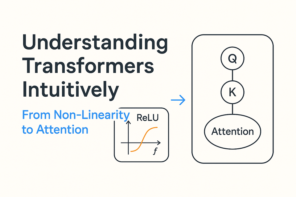
Understanding Transformers Intuitively: From Non-Linearity to Attention

In the rapidly evolving landscape of artificial intelligence, few innovations have made as profound an impact as the Transformer architecture. Since its introduction in the landmark 2017 paper "Attention Is All You Need," Transformers have revolutionized natural language processing, computer vision, and numerous other domains. Yet despite their ubiquity—powering everything from ChatGPT to image generation models—many practitioners and enthusiasts find Transformers conceptually challenging to grasp. The intricate mathematics and complex architecture can obscure the elegant intuitions that make these models so powerful.

This blog aims to demystify Transformers by building an intuitive understanding from the ground up. Rather than diving straight into the mathematical complexities, we'll start with fundamental concepts like non-linearity in neural networks—the essential property that allows these models to learn complex patterns. We'll explore how simple activation functions serve as "gates" that enable neural networks to bend and shape information, creating the foundation upon which more sophisticated architectures like Transformers are built.

As we progress, we'll unpack the attention mechanism—the revolutionary concept that allows Transformers to process information in parallel while maintaining awareness of context and relationships between elements. Through clear explanations and visual aids, we'll see how Transformers use attention to focus on what matters in data, whether it's understanding the relationship between words in a sentence or identifying important features in an image.

By the end of this journey, you'll have developed not just a surface-level familiarity with Transformers, but a deeper intuitive grasp of how and why they work. Whether you're a developer looking to implement these models, a researcher seeking to innovate upon them, or simply a curious mind fascinated by AI, this exploration will equip you with the conceptual tools to understand one of the most important architectural innovations in modern machine learning.

Let's begin our exploration by understanding a fundamental concept that underpins all neural networks: non-linearity, and why it's so crucial for learning complex relationships in data.

The Foundation: Non-Linearity in Neural Networks

At the heart of every neural network, including the sophisticated Transformer architecture, lies a fundamental concept that enables these models to learn complex patterns: non-linearity. To truly understand Transformers, we must first grasp why non-linearity is so crucial in neural computation.

Imagine trying to model the relationship between the number of hours studied and exam scores. In the simplest case, this might be a linear relationship: each additional hour of study adds a fixed number of points to your score. Mathematically, we express this as y = mx + c, where y is the exam score, x is the hours studied, m is the rate of improvement per hour, and c is some baseline score. This is a linear function—a straight line on a graph—and it's relatively simple to understand and compute.

But real-world relationships are rarely so straightforward. Perhaps the first few hours of studying yield dramatic improvements, but after a certain point, additional hours yield diminishing returns as fatigue sets in. Or maybe there's a threshold effect where studying less than a certain amount yields almost no benefit, but once you cross that threshold, your understanding rapidly improves. These are non-linear relationships—they can't be represented by a simple straight line.

Neural networks face a similar challenge. When we build a neural network layer, the basic operation is fundamentally linear: we multiply inputs by weights, add a bias term, and get an output (y = wx + b). If we were to stack multiple layers that only performed these linear operations, something interesting would happen: no matter how many layers we added, the entire network would still only be capable of learning linear relationships. This is because a composition of linear functions is still just a linear function.

This is where activation functions come into play. An activation function introduces non-linearity into the network by "bending" the output of a linear operation. The most commonly used activation function today is ReLU (Rectified Linear Unit), which is defined simply as f(x) = max(0, x). This function passes through positive values unchanged but converts all negative values to zero. This creates a "kink" in the function at x = 0, breaking the linearity. Looking at the graph provided in our conversation, we can see this effect clearly.

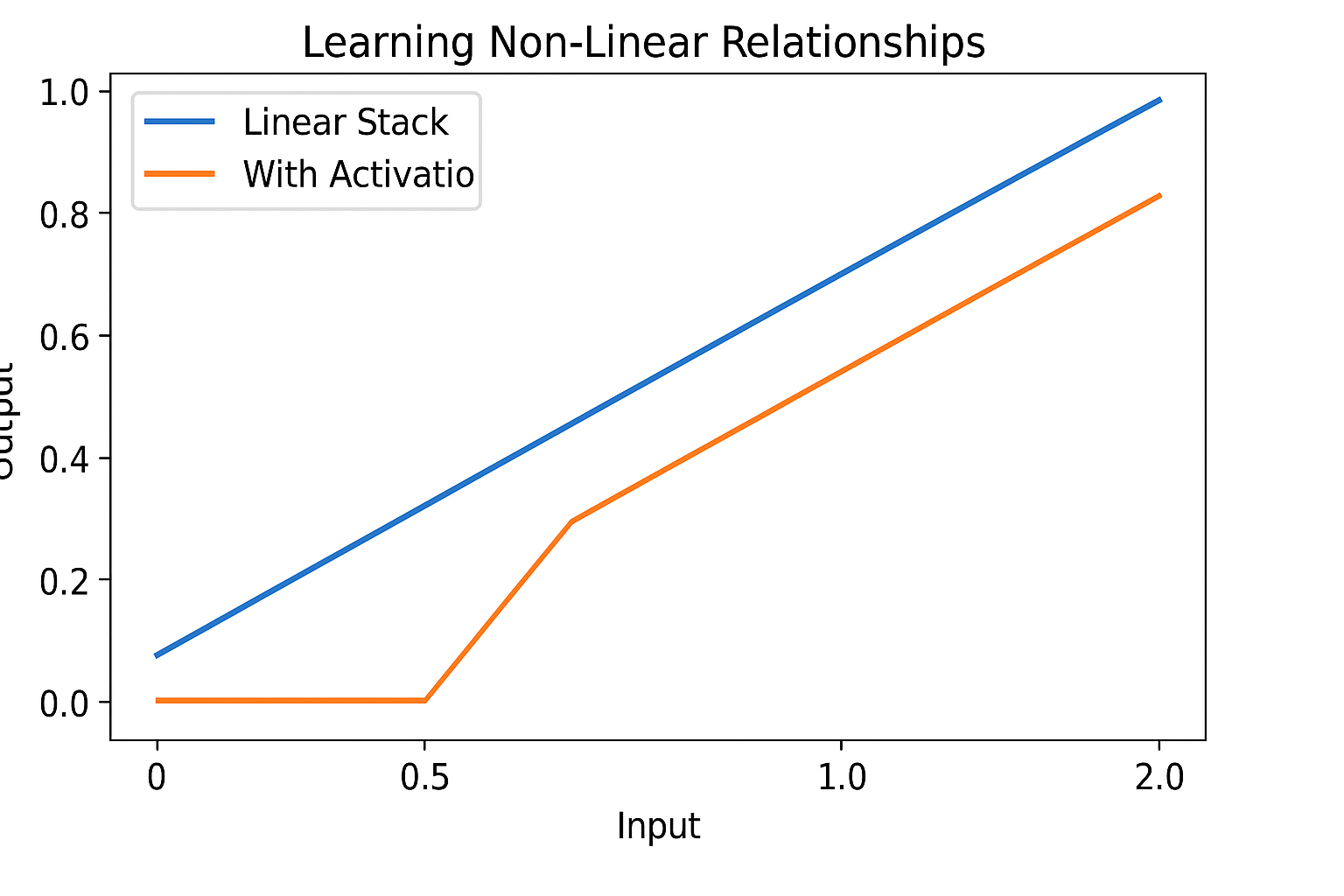
Figure: Comparison of a linear stack vs. a stack with a non-linear activation function (e.g., ReLU).

The blue line represents a purely linear stack of operations - notice how it forms a straight line. No matter how many linear layers we stack, the relationship remains linear. The orange line shows what happens when we introduce a non-linear activation function. Notice how the orange line remains flat at zero until a certain input threshold, then begins to rise—but not at the same rate as the linear function. This simple "bending" of the line is what gives neural networks their expressive power.

When we stack multiple layers with non-linear activations between them, something remarkable happens. The network can now approximate virtually any function, no matter how complex. This is formalized in the Universal Approximation Theorem, which states that a neural network with just a single hidden layer and a non-linear activation function can approximate any continuous function to arbitrary precision, given enough neurons.

To make this concrete, let's consider a simple example. Imagine we want to model the exclusive OR (XOR) function, which outputs 1 when exactly one of its two inputs is 1, and 0 otherwise. This is a classic example of a function that cannot be represented by a single linear boundary. No matter how you try to draw a straight line on a graph of XOR inputs and outputs, you cannot separate the 1s from the 0s. But with a non-linear activation function and at least one hidden layer, a neural network can learn to represent this function perfectly.

This ability to model non-linear relationships is what allows neural networks to learn complex patterns in data, whether it's recognizing objects in images, understanding the nuances of language, or predicting intricate time series. And as we'll see, this same principle extends to Transformers, where non-linearity plays a crucial role in the model's ability to understand the complex relationships between elements in a sequence.

In the next section, we'll explore activation functions in more detail, understanding how they act as "gates" that control the flow of information through a neural network, and how the choice of activation function can significantly impact a model's learning capabilities.

Activation Functions: The Gates of Neural Networks

Having established the critical importance of non-linearity in neural networks, let's delve deeper into the mechanisms that introduce this non-linearity: activation functions. These mathematical operations serve as the "gates" of neural networks, controlling how information flows through the network and enabling it to learn complex patterns.

An activation function takes the output of a linear operation (weights multiplied by inputs plus a bias) and transforms it before passing it to the next layer.

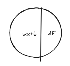
Figure: A simple representation of a neuron, combining a linear operation (wx+b) with a non-linear activation function (AF).

The choice of activation function significantly impacts how a neural network learns and performs. In our conversation, we explored several common activation functions, each with its own characteristics and use cases.

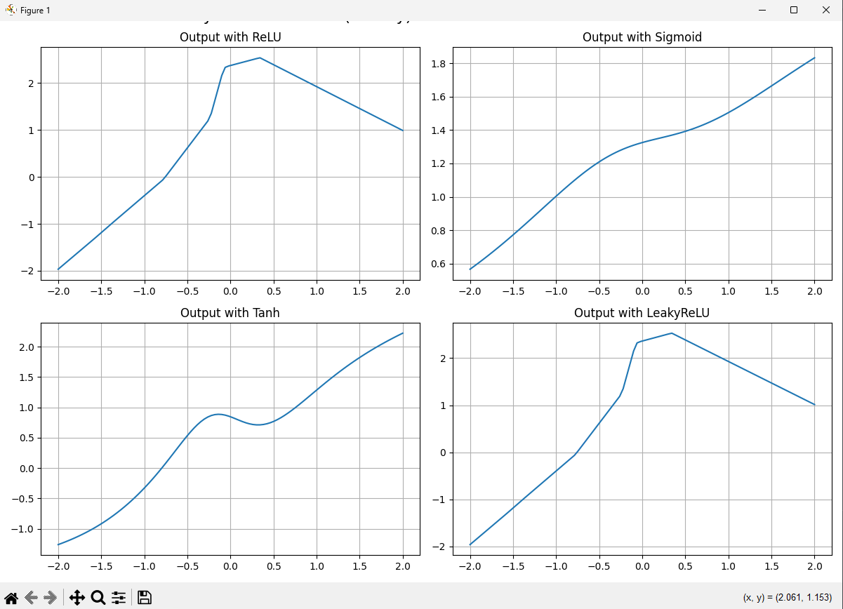
Figure: Comparison of common activation functions (ReLU, Sigmoid, Tanh, and LeakyReLU) showing how they transform input values.

# Code to generate activation function visualizations
import numpy as np
import matplotlib.pyplot as plt

# Define activation functions
def relu(x): return np.maximum(0, x)
def sigmoid(x): return 1 / (1 + np.exp(-x))
def tanh(x): return np.tanh(x)
def leaky_relu(x): return np.where(x > 0, x, 0.01 * x)

# Input values
X = np.linspace(-2, 2, 100).reshape(-1, 1)

# Plot results
plt.figure(figsize=(12, 8))
activations = {
    "ReLU": relu,
    "Sigmoid": sigmoid,
    "Tanh": tanh,
    "LeakyReLU": leaky_relu
}

for i, (name, fn) in enumerate(activations.items()):
    output = fn(X)
    plt.subplot(2, 2, i + 1)
    plt.plot(X, output)
    plt.title(f"Output with {name}")
    plt.grid(True)

plt.tight_layout()
plt.suptitle("Activation Functions Comparison", fontsize=16, y=1.02)
plt.show()

The Rectified Linear Unit (ReLU) has become the default choice for many neural networks, including Transformers. Its formula is elegantly simple: f(x) = max(0, x). For any positive input, ReLU outputs that same value; for any negative input, it outputs zero. This creates a simple "gate" that allows positive signals to pass through unchanged while blocking negative signals entirely. Despite its simplicity, ReLU offers several advantages. It computes quickly, doesn't saturate for positive values (meaning gradients don't vanish), and creates sparse activations where many neurons output zero, encouraging specialization among neurons.

The Sigmoid function, defined as \( f(x) = \frac{1}{1 + e^{-x}} \), squashes any input into a range between 0 and 1. This S-shaped curve approaches 0 for very negative inputs and approaches 1 for very positive inputs. Sigmoid was once widely used in hidden layers but has fallen out of favor due to the "vanishing gradient problem"—when inputs are far from zero, the gradient becomes very small, making learning difficult. However, Sigmoid remains valuable for output layers in binary classification tasks, where we need to predict probabilities between 0 and 1.

TanH (hyperbolic tangent) is similar to Sigmoid but ranges from -1 to 1 instead of 0 to 1. This zero-centered output can be advantageous in some contexts, particularly in recurrent neural networks. Softmax, meanwhile, is not applied element-wise like the others but instead converts a vector of numbers into a probability distribution, making it ideal for multi-class classification output layers.

More recent architectures have introduced variations like Leaky ReLU (which allows a small gradient for negative inputs), ELU (Exponential Linear Unit), GELU (Gaussian Error Linear Unit, used in models like BERT and GPT), and Swish (x * sigmoid(x)). Each of these attempts to address specific limitations of earlier activation functions, offering improved training stability or performance in certain contexts.

What's fascinating about activation functions is that they don't change during training. As pointed out in our conversation, when a neural network learns, it's not modifying the activation functions themselves—it's adjusting the weights and biases that control what flows into these functions. This is a profound insight: the activation function is like a gate, and the model learns how to open and close that gate by shaping what flows into it.

To illustrate this, consider a neural network learning to recognize smiles in images. The network doesn't change how ReLU works; instead, it adjusts weights so that when smile-like features are present, the input to ReLU becomes positive (allowing the signal to pass), and when such features are absent, the input becomes negative (blocking the signal). Over time, different neurons in the network specialize in detecting different features—some might activate for upturned corners of the mouth, others for visible teeth, and so on.

This specialization emerges naturally during training through the process of gradient descent and backpropagation. When the network makes a prediction error, the gradient of the loss with respect to each weight indicates whether that weight should increase or decrease to improve performance. The learning rate controls how quickly these adjustments occur. Through many iterations of this process, the network gradually learns to control the gates in a way that produces the desired output.

The choice of activation function can significantly impact this learning process. For instance, if we had used Sigmoid instead of ReLU in our hidden layers, every neuron would always activate at least a little bit (since Sigmoid never reaches exactly 0), making it harder for neurons to specialize. The network might still learn, but training would likely be slower and less effective.

In Transformer architectures, activation functions play a crucial role in the feed-forward networks that process the output of attention mechanisms. Typically, these use ReLU or GELU activations to introduce non-linearity into what would otherwise be purely linear transformations. This non-linearity is essential for the model to learn complex relationships between elements in a sequence, whether they're words in a sentence or patches in an image.

As we move forward to explore attention mechanisms and the full Transformer architecture, keep in mind this fundamental insight: at every stage, non-linear activation functions serve as gates that allow the network to shape and control information flow, enabling it to learn the complex patterns that make modern AI so powerful.

From Basic Neural Networks to Attention

As we've explored the foundations of neural networks through non-linearity and activation functions, we're now ready to make the conceptual leap to one of the most powerful innovations in deep learning: attention mechanisms. These mechanisms form the heart of Transformer models and represent a fundamental shift in how neural networks process sequential data.

Traditional neural networks, including convolutional neural networks (CNNs) and recurrent neural networks (RNNs), have inherent limitations when dealing with sequences like sentences or time series. CNNs excel at capturing local patterns but struggle with long-range dependencies. RNNs process sequences step by step, maintaining a hidden state that carries information forward, but this sequential processing creates bottlenecks: information from the beginning of a sequence can get diluted by the time the network reaches the end, and the sequential nature prevents parallelization.

Attention mechanisms were developed to address these limitations. The core intuition behind attention is remarkably human: when processing information, not all parts are equally important. When you read a sentence, you naturally focus on certain words more than others to understand the meaning. Similarly, attention mechanisms allow neural networks to "focus" on different parts of the input when producing each part of the output.

The breakthrough of the Transformer architecture was to show that "attention is all you need" – that is, a model based entirely on attention mechanisms, without recurrence or convolution, could outperform previous architectures on sequence processing tasks[1]. This was revolutionary because it allowed for much more parallelization (speeding up training and inference) while also capturing long-range dependencies more effectively.

At the heart of the Transformer's attention mechanism is the Query, Key, Value (Q, K, V) paradigm. This conceptual framework helps us understand how attention works:

1. Query (Q): Represents what we're looking for or what we're interested in
2. Key (K): Represents what we have available or what we're comparing against
3. Value (V): Represents the actual content we want to retrieve or focus on

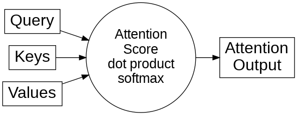
Figure: The attention mechanism in Transformers, showing how Query, Keys, and Values interact through dot products and softmax to produce the attention output.

To make this concrete, imagine you're at a library looking for books on a specific topic. Your query is the topic you're interested in. Each book has a title and keywords (the keys) that you compare against your query. When you find books with relevant keys, you take their content (the values). Books with more relevant keys get more of your attention.

In a Transformer, for each position in a sequence (like each word in a sentence), the model computes query, key, and value vectors through learned linear transformations. It then computes attention scores by comparing each query with all keys. These scores determine how much each value contributes to the output for that position.

The mathematical operation is elegant: the attention score between a query and a key is their dot product (a measure of similarity)[3], scaled by the square root of the dimension of the key vectors, and then passed through a softmax function to get a probability distribution. These probabilities are used to take a weighted sum of the value vectors, producing the attention output.

Side Note: Understanding Dot Products in Attention Mechanisms

When discussing attention mechanisms in Transformers, we frequently mention that attention scores are calculated using dot products between query and key vectors. But what exactly is a dot product, and why is it useful for measuring similarity between vectors?

The dot product[3] of two vectors u and v is defined as:

u⋅v = |u||v|cosθ

Where |u| and |v| are the magnitudes (lengths) of the vectors, and θ is the angle between them.

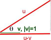
It's perhaps easiest to visualize the dot product's use as a similarity measure when |v| = 1 (i.e., v is a unit vector), as shown in the diagram above. In this case:

cosθ = \( \mathbf{u} \cdot \mathbf{v} = |\mathbf{u}| |\mathbf{v}| \cos\theta \)

Looking at the diagram, we can understand several important properties:

• When θ = 0° and cosθ = 1 (the vectors are pointing in the same direction), the dot product equals the magnitude of u. This represents maximum similarity.
• When θ = 90° and cosθ = 0 (the vectors are perpendicular or orthogonal), the dot product equals 0. This represents no similarity in direction.
• When θ = 180° and cosθ = -1 (the vectors are pointing in opposite directions), the dot product equals the negative of the magnitude of u. This represents maximum dissimilarity.

In general, cosθ tells you the similarity in terms of the direction of the vectors. This property holds as the number of dimensions increases, making the dot product an excellent similarity measure in multi-dimensional space.

In the context of Transformer attention mechanisms, when we compute the dot product between a query vector and a key vector, we're essentially measuring how similar or aligned these vectors are. Higher dot product values indicate greater similarity, which translates to higher attention scores. This is why the dot product is fundamental to how attention works - it allows the model to focus on elements that are most relevant (similar) to what it's looking for.

When these dot products are scaled and passed through a softmax function to create a probability distribution, they become the weights that determine how much each value vector contributes to the output. This elegant use of vector similarity is at the heart of what makes Transformer attention mechanisms so effective.

What makes this mechanism so powerful is that it allows direct connections between any two positions in a sequence, regardless of how far apart they are. This means that long-range dependencies can be captured just as easily as short-range ones. Additionally, since the attention computation for each position is independent, the entire process can be parallelized, making Transformers much more efficient to train than RNNs.

Self-attention, the specific form used in Transformers, is particularly interesting. In self-attention, the queries, keys, and values all come from the same source – the input sequence itself. This allows each position to attend to all positions, including itself. The result is that each output element contains information from the entire input sequence, weighted by relevance.

Why does self-attention scale better than recurrence? In an RNN, information from the beginning of a sequence must pass through every intermediate step to reach the end, potentially getting diluted or lost along the way. The computational path length between any two positions grows linearly with their distance. In contrast, self-attention creates direct paths between any two positions, regardless of distance. This constant path length means that even very long-range dependencies can be captured effectively.

The multi-head attention mechanism in Transformers takes this a step further by running multiple attention operations in parallel, each with different learned projections. This allows the model to attend to information from different representation subspaces and different positions, capturing various aspects of the relationships between elements in the sequence.

As we move forward to examine the complete Transformer architecture, keep in mind that this attention mechanism – this ability to focus on what matters across an entire sequence – is what gives Transformers their remarkable power and flexibility.

The Transformer Architecture Explained

Now that we understand the power of attention mechanisms, let's examine how they're integrated into the complete Transformer architecture. The diagram provided in our conversation offers a visual representation of the Transformer blocks, which form the core of this revolutionary architecture.

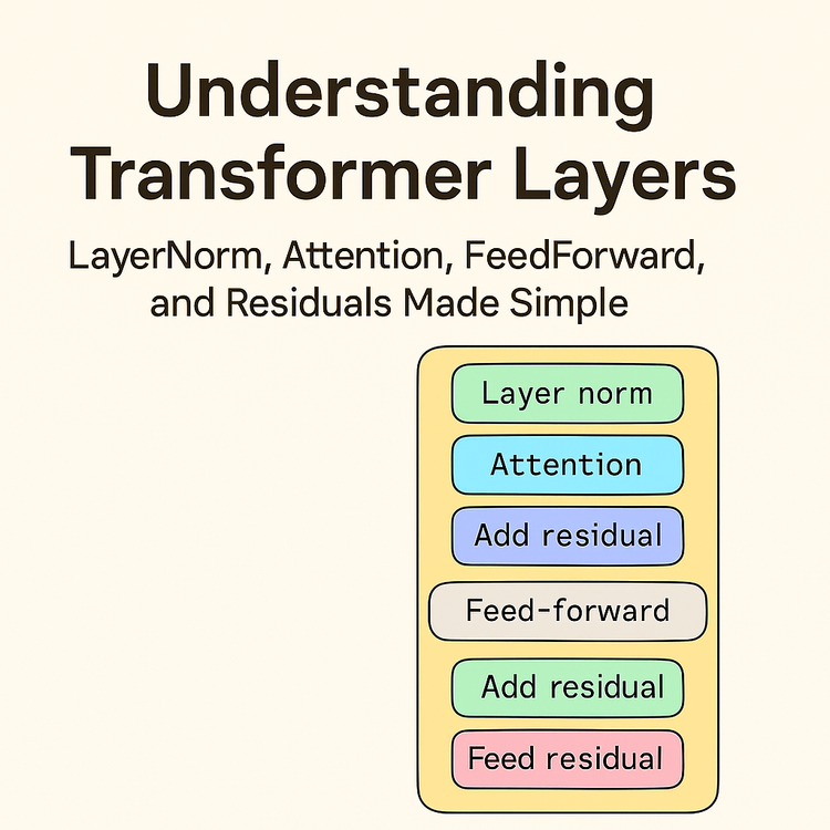
A Transformer consists of a stack of identical layers, each containing two main sub-layers: a multi-head self-attention mechanism and a position-wise feed-forward network. Let's break down each component to understand how they work together.

At the input level, Transformers first convert tokens (such as words in a sentence) into embeddings—dense vector representations that capture semantic meaning. Unlike models that use precomputed embeddings like Word2Vec or Doc2Vec, Transformers learn embeddings jointly with the model during training. Since Transformers process all elements of a sequence in parallel rather than sequentially, they need a way to encode position information. This is achieved through positional encodings, which are added to the input embeddings to give the model information about the relative or absolute position of each token in the sequence.

Looking at the diagram, we can see the flow of information through a Transformer block. The attention mechanism computes weighted combinations using dot products (Q · K), not simple wx + b layers. The feedforward network applies wx + b and non-linear activations after attention is done. This distinction is important for understanding how Transformers process information.

The attention mechanism, as we've discussed, allows each position to attend to all positions in the previous layer. The attention mechanism itself is composed of dot products and softmax (which is a non-linearity), but the deeper non-linear transformations happen in the feedforward layers. In practice, Transformers use multi-head attention, which runs multiple attention operations in parallel. Each "head" can focus on different aspects of the relationships between elements, allowing the model to jointly attend to information from different representation subspaces.

After the attention mechanism, the output passes to what the diagram labels as "non attention neuron"—this is the position-wise feed-forward network. This component consists of two linear transformations with a non-linear activation function (typically ReLU or GELU) in between:

FFN(x) = \( \max(0, xW_1 + b_1)W_2 + b_2 \)

This feed-forward network is applied to each position independently and identically, using the same weights across all positions. It transforms the attention output into a representation that can be processed by the next layer or used for final predictions.

One crucial aspect of the Transformer architecture not explicitly shown in our simplified diagram is the use of residual connections and layer normalization. After each sub-layer (both the attention mechanism and the feed-forward network), the Transformer adds the input to the sub-layer's output (a residual connection) and then applies layer normalization. These techniques help with training stability and allow for deeper networks.

The complete Transformer architecture typically includes an encoder stack and a decoder stack, each composed of multiple identical layers as described above. The encoder processes the input sequence, while the decoder generates the output sequence. In the decoder, an additional attention layer allows it to attend to the encoder's output.

What makes this architecture so powerful? Several key factors:

1. Parallelization: Unlike RNNs, which process sequences step by step, Transformers process all elements simultaneously, allowing for much more efficient training and inference.
2. Long-range dependencies: The attention mechanism creates direct paths between any two positions, regardless of their distance, making it easier to capture long-range dependencies.
3. Capacity: The combination of multiple attention heads and deep stacks of layers gives Transformers enormous capacity to model complex relationships.
4. Flexibility: The same basic architecture can be applied to a wide range of tasks, from language translation to image recognition, with minimal task-specific modifications.

The diagram in our conversation emphasizes an important point: "These transformer blocks are hidden layers. The output of input first goes to attention and then to non attention neuron as shown and its output goes to next block (first to attention and then to regular FF calculation)." This captures the essence of how information flows through a Transformer—each block processes the output of the previous block, with attention mechanisms and feed-forward networks working together to transform the representation at each step.

This architecture has proven remarkably effective across a wide range of tasks and has spawned numerous variations and improvements. Models like BERT, GPT, T5, and many others are all based on the Transformer architecture, with modifications to suit specific applications. The fundamental principles, however, remain the same: attention mechanisms allow the model to focus on relevant information, while feed-forward networks and non-linear activations provide the capacity to learn complex transformations.

Self-Attention: The Heart of Transformers

Having explored the overall Transformer architecture, let's dive deeper into what many consider the most innovative aspect of Transformers: the self-attention mechanism. This mechanism is truly the heart of the Transformer, enabling it to model complex relationships between elements in a sequence with remarkable effectiveness.

Self-attention, at its core, is about relating different positions of a single sequence to compute a representation of that sequence. Unlike traditional attention used in encoder-decoder architectures where the decoder attends to the encoder's output, in self-attention, the queries, keys, and values all come from the same source. This allows each element in a sequence to attend to every other element, including itself, creating a rich representation that captures the full context.

To understand self-attention intuitively, consider how we understand language. When you read the sentence "The animal didn't cross the street because it was too wide," you naturally link "it" with "street" rather than "animal." You do this by attending to relevant parts of the sentence to resolve the reference. Self-attention works similarly, allowing the model to create links between related words regardless of their distance in the sequence.

The mathematics of self-attention, while elegant, can be simplified to understand the core intuition. For each position in the sequence:

1. We compute query, key, and value vectors through learned linear transformations.
2. For each query, we compute its dot product with all keys to get attention scores.
3. We scale these scores and apply a softmax to get a probability distribution.
4. We use these probabilities to take a weighted sum of the value vectors.

This process creates an output where each position contains information from the entire sequence, weighted by relevance. The multi-head attention used in Transformers runs this process multiple times in parallel with different learned projections, allowing the model to attend to different aspects of the relationships simultaneously.

One of the most illuminating ways to understand self-attention is to visualize the attention weights—the probabilities that determine how much each position contributes to each output. When visualized as a matrix, with rows representing queries and columns representing keys, we can see patterns emerge that reveal how the model is relating different elements.

For example, in a language model, we might see that articles ("the", "a") strongly attend to the nouns they modify, verbs attend to their subjects and objects, and pronouns attend to their antecedents. These patterns emerge naturally during training as the model learns to solve tasks that require understanding these relationships.

What makes self-attention particularly powerful is its ability to handle long-range dependencies. In traditional sequence models like RNNs, information from the beginning of a sequence must pass through every intermediate step to reach the end, potentially getting diluted along the way. In contrast, self-attention creates direct paths between any two positions, regardless of their distance. This means that even in very long sequences, relationships between distant elements can be captured effectively.

Another advantage of self-attention is its interpretability. By examining the attention weights, we can often gain insights into how the model is processing information. This has made Transformers not just powerful models but also valuable tools for understanding language and other sequential data.

The scaling of self-attention is another important aspect mentioned in our conversation. Traditional recurrent models scale poorly with sequence length because they process elements sequentially. Self-attention, on the other hand, processes all elements in parallel, making it much more efficient for training. While the attention computation itself scales quadratically with sequence length (as each position attends to all positions), this is offset by the benefits of parallelization and the ability to capture long-range dependencies.

Recent research has focused on addressing this quadratic scaling issue, with various approaches like sparse attention patterns, low-rank approximations, and other techniques that maintain the benefits of self-attention while reducing computational complexity for very long sequences.

As we continue to explore Transformers, remember that this self-attention mechanism—this ability for each element to directly interact with every other element—is what gives these models their remarkable capacity to understand context and relationships in sequential data.

Understanding Logits in Transformers: From Raw Outputs to Probabilities

To complete our intuitive understanding of Transformers, let's explore an important concept that bridges the model's internal representations with its final predictions: logits. This concept is crucial for understanding how Transformer models actually make decisions[2].

Logits are the raw, unnormalized outputs of a neural network before any final activation function (like softmax) is applied. The term comes from the logistic function in statistics, but in deep learning, we use it more broadly to refer to these pre-normalized scores.

What Are Logits and Why Do They Matter?

In the context of Transformers and other neural networks, logits represent the model's "confidence" or "evidence" for each possible output class, but in a form that's not yet scaled to be directly interpretable as probabilities. They're essentially the direct output from the final linear layer of the network.

Let's understand this with a concrete example[2]:

Imagine we've built a Transformer model to classify images as either cats or dogs. When we feed an image into our model, the final layer outputs two numbers (logits) - one score for "cat" and one for "dog".

For a particular image, our model might output these logits:

• Cat: 16.917
• Dog: 0.772

The higher value (16.917 for cat) suggests the model believes this image contains a cat rather than a dog. But these raw numbers aren't easily interpretable on their own. How confident is the model exactly? Is 16.917 very confident or just slightly confident?

This is where normalization comes in. By applying the softmax function to these logits, we convert them into probabilities that sum to 1:

σ(z)j = \( \frac{e^{z_j}}{\sum_{k=1}^K e^{z_k}} \) for \( j = 1, \dots, K \)

For our example:

• P(cat) = \( \frac{e^{16.917}}{e^{16.917} + e^{0.772}} \approx 0.9999 \)
• P(dog) = \( \frac{e^{0.772}}{e^{16.917} + e^{0.772}} \approx 0.0001 \)

Now we can clearly see that the model is 99.99% confident this image contains a cat.

Logits Reveal Model Uncertainty

Let's look at another example with our cat-dog classifier. For a different image, the model outputs these logits:

• Cat: 1.004
• Dog: 0.709

Converting to probabilities:

• P(cat) =\( \frac{e^{1.004}}{e^{1.004} + e^{0.709}} \approx 0.5732 \)
• P(dog) = \( \frac{e^{0.709}}{e^{1.004} + e^{0.709}} \approx 0.4268 \)

In this case, although the model still predicts "cat," it's much less certain - only about 57% confident. This is valuable information that would be lost if we only looked at the final classification without examining the logits or their normalized probabilities.

Logits in Transformer Models

In Transformer models like BERT or GPT, the final layer typically produces logits for each token in the vocabulary (which can be tens of thousands of values). For language models, these logits represent the model's prediction for the next token in a sequence.

The process works like this:

1. The input passes through all the Transformer layers (attention mechanisms and feed-forward networks)
2. The final layer produces a vector of logits for each position in the sequence
3. These logits are converted to probabilities using softmax
4. The token with the highest probability is selected (or in generation tasks, sampled according to these probabilities)

Why We Don't Apply Non-Linearity to Logits

An interesting point mentioned in our conversation is that we typically don't apply non-linear activation functions to logits before the final softmax. Why is this?

The reason is that logits represent the raw, unbiased evidence the model has accumulated for each class. Applying a non-linearity before softmax would distort this evidence, potentially cutting off information right before the final prediction is made.

While softmax introduces non-linearity to the vector of logits, it differs from activation functions like ReLU that are applied element-wise. Softmax operates on the entire vector at once, transforming it into a probability distribution where all values sum to 1. This preserves the full range of the model's predictions while making them interpretable as probabilities.

Logits and Loss Functions

Logits also play a crucial role in how we train neural networks. Many common loss functions for classification tasks, like cross-entropy loss, work directly with logits rather than probabilities. This approach is numerically more stable and avoids potential issues with very small probability values.

In the context of Transformers, understanding logits helps us grasp how these models make decisions and how we can interpret their outputs. By examining the raw logits or their normalized probabilities, we gain insight into not just what the model predicts, but also how confident it is in those predictions - a crucial aspect of building reliable AI systems.

Visualizing Transformers: Making the Concepts Concrete

To solidify our understanding of Transformers, let's examine some visual representations of the key concepts we've discussed. These visualizations help make abstract ideas more concrete and intuitive.

Non-Linear Relationships

This graph powerfully illustrates the difference between linear and non-linear functions in neural networks. The blue line represents a purely linear stack of operations - notice how it forms a perfect straight line from the origin to the upper right. No matter how many linear layers we stack on top of each other, the relationship remains linear.

The orange line, however, shows what happens when we introduce a non-linear activation function (likely ReLU in this case). Notice how it remains flat at zero until the input reaches approximately 0.5, then begins to rise - but not at the same rate as the linear function. This "kink" in the line at x=0.5 is the non-linearity that gives neural networks their power.

This simple visualization demonstrates why non-linear activation functions are essential. Without them, neural networks would be limited to learning only linear relationships, regardless of how deep they are. The non-linearity allows the network to approximate complex functions by combining these bent lines in sophisticated ways.

Transformer Architecture

The Transformer architecture can be visualized as a series of blocks, each containing two main components: an attention mechanism and a feed-forward network. From the conversation, we saw a diagram that illustrates this structure clearly.

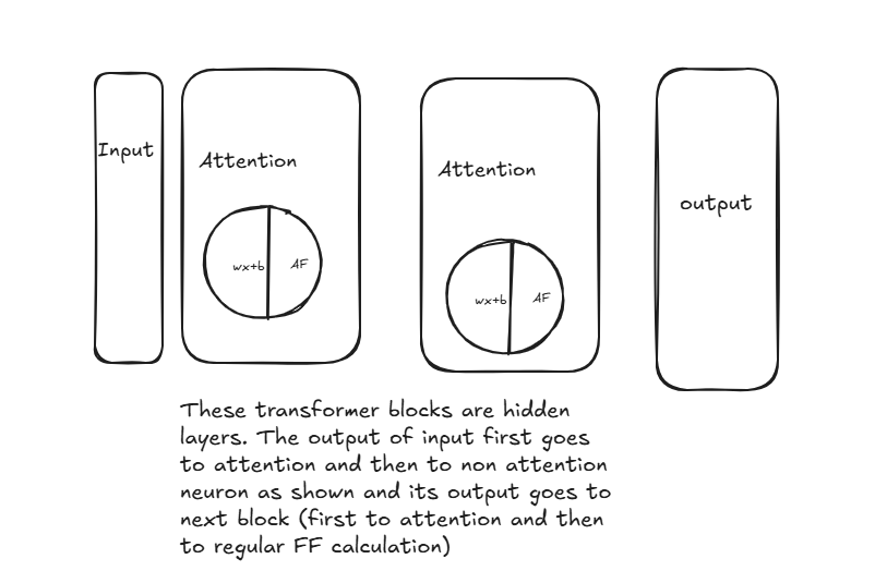
Figure: A simplified view of Transformer blocks, showing the flow from input through attention and feed-forward layers to the output.

In the diagram, we see the flow of information through a Transformer block:

1. Input Layer: The sequence data first enters the Transformer.
2. Attention Mechanism: The input goes to an attention block, represented by a circle divided into two parts labeled "wx+b" (the linear transformation) and "AF" (activation function). This visual representation captures how attention combines linear operations with non-linear activations.
3. Feed-Forward Network: After the attention mechanism, the output passes to what was labeled as "non-attention neuron" - this is the position-wise feed-forward network that applies the same transformation to each position independently.
4. Output: The processed information then flows to the next block or to the final output layer.

The diagram emphasizes an important aspect of Transformer architecture: "These transformer blocks are hidden layers. The output of input first goes to attention and then to non-attention neuron as shown and its output goes to next block (first to attention and then to regular FF calculation)."

This structure allows Transformers to process information in a highly parallel manner while still capturing complex relationships between elements in a sequence. The attention mechanism enables each position to focus on relevant parts of the input, while the feed-forward network provides the capacity to transform this information in powerful ways.

Self-Attention Visualization

While not explicitly shown in our images, self-attention can be visualized as a matrix where each cell represents how much one position attends to another. In language models, this often reveals interpretable patterns:

• Articles ("the", "a") strongly attend to the nouns they modify
• Verbs attend to their subjects and objects
• Pronouns attend to their antecedents

These attention patterns emerge naturally during training as the model learns to solve tasks that require understanding relationships between elements in a sequence.

By visualizing these concepts, we can develop a more intuitive understanding of how Transformers work and why they're so effective at processing sequential data.

Conclusion: The Transformative Power of Transformers

Throughout this blog post, we've taken a journey from the fundamental concepts of neural networks to the sophisticated architecture of Transformers. By building our understanding layer by layer, we've developed an intuitive grasp of how these powerful models work and why they've revolutionized artificial intelligence.

We began with the concept of non-linearity—the essential property that allows neural networks to learn complex patterns in data. We saw how simple activation functions like ReLU introduce "bends" in otherwise linear operations, enabling networks to approximate any function given sufficient capacity. This non-linearity is the foundation upon which all advanced neural architectures, including Transformers, are built.

We then explored activation functions in more detail, understanding how they act as "gates" that control the flow of information through a network. The model doesn't change these gates during training; instead, it learns to shape what flows into them by adjusting weights and biases. This insight helps demystify how neural networks learn to recognize complex patterns despite using relatively simple activation functions.

From there, we made the leap to attention mechanisms—the revolutionary concept that allows Transformers to process information in parallel while maintaining awareness of context and relationships. We saw how the Query, Key, Value paradigm enables each position in a sequence to focus on relevant parts of the input, regardless of distance. This ability to create direct paths between any two positions is what gives Transformers their remarkable power to capture long-range dependencies.

We examined the complete Transformer architecture, understanding how attention mechanisms and feed-forward networks work together in a series of identical layers to transform input representations. The parallelization enabled by this architecture, combined with its capacity to model complex relationships, explains why Transformers have been so successful across a wide range of tasks.

We dove deeper into self-attention—the heart of the Transformer—and visualized key concepts to make them more concrete and intuitive. We also explored the concept of logits and how they bridge the model's internal representations with its final predictions, providing insight into not just what the model predicts but also how confident it is in those predictions.

The impact of Transformers on artificial intelligence cannot be overstated. They've enabled breakthroughs in natural language processing, with models like BERT, GPT, and T5 achieving unprecedented performance on a wide range of tasks. They've been adapted for computer vision, where models like Vision Transformer (ViT) have challenged the dominance of convolutional architectures. They've enabled multimodal models that can process and generate both text and images. And they continue to evolve, with researchers finding ways to make them more efficient, more capable, and applicable to new domains.

Hyperparameters in Transformers: The Control Panel of Model Design

Before we conclude our exploration of Transformers, let's discuss an important aspect of these models that significantly impacts their performance: hyperparameters. Understanding hyperparameters is essential for anyone looking to work with or implement Transformer models.

What Are Hyperparameters?

Hyperparameters are configuration settings that the model developer establishes before training begins. Unlike the model's weights and biases that are learned during training, hyperparameters are set manually and remain fixed throughout the training process.

Think of hyperparameters like a pilot's control panel in an airplane. Before takeoff, the pilot sets various parameters that will govern the flight - altitude, speed, route - and these settings determine how the journey will unfold. Similarly, a model developer sets hyperparameters before training begins, and these settings determine how the model will be structured and how it will learn.

Another helpful analogy is that of a water flow engineer adjusting valves in a complex system. By opening some valves more than others, the engineer controls how much water flows through different parts of the system. In the same way, hyperparameters control the "flow" of information and learning in a Transformer model.

Key Hyperparameters in Transformer Models

Architectural Hyperparameters

1. Number of Layers: This determines how many encoder or decoder blocks the model has. More layers allow for more complex representations but require more computation. It's like deciding how many floors to build in a skyscraper - more floors provide more space but cost more to build and maintain.
2. Hidden Size: This controls the dimensionality of the vectors used throughout the model. Larger hidden sizes can capture more information but require more memory. This is similar to deciding the width of water pipes - wider pipes allow more water to flow but require more materials and space.
3. Number of Attention Heads: Multi-head attention splits attention into multiple "heads" that can focus on different aspects of the input. More heads can capture more diverse relationships but increase computational requirements. Think of this as having multiple pilots monitoring different aspects of the flight simultaneously.
4. Feed-Forward Network Size: The dimensionality of the inner layer in the feed-forward networks. Larger sizes provide more capacity for complex transformations, like having more powerful engines in an airplane.

Training Hyperparameters

1. Learning Rate: Controls how quickly the model updates its parameters during training. Too high, and training becomes unstable; too low, and training becomes inefficiently slow. This is like controlling the speed of an airplane - too fast might be dangerous, too slow wastes time.
2. Batch Size: The number of examples processed together. Larger batches provide more stable gradient estimates but require more memory. This is similar to deciding how many passengers to board on each flight.
3. Dropout Rate: Controls the probability of randomly "dropping" neurons during training to prevent overfitting. It's like occasionally closing certain valves in a water system to ensure the system doesn't become too dependent on any single path.

The Impact of Hyperparameters on Model Performance

Hyperparameters create important trade-offs between:

1. Model Size: Larger models can learn more complex patterns but require more resources.
2. Training/Inference Speed: Faster models are more practical but may sacrifice performance.
3. Accuracy/Performance: Better performance is the goal, but often comes at the cost of larger, slower models.

Consider the difference between models like BERT and DistilBERT. DistilBERT uses fewer layers and a smaller hidden size than BERT, making it 60% faster while retaining 97% of BERT's performance. This is like designing a more fuel-efficient airplane that sacrifices a small amount of speed for significant savings in fuel consumption.

Finding the Right Hyperparameters

Selecting hyperparameters is both an art and a science:

1. Start with Established Configurations: Models like BERT, GPT, and T5 have well-documented hyperparameter settings that work well for many tasks.
2. Hyperparameter Search: Techniques like grid search, random search, or Bayesian optimization can systematically explore the hyperparameter space.
3. Consider Your Resources: Choose hyperparameters that fit within your computational constraints, just as a pilot must consider fuel capacity when planning a flight.

Understanding hyperparameters helps us appreciate the flexibility of Transformer architectures, which can scale from small, efficient models to massive, state-of-the-art systems simply by adjusting these control settings. By thoughtfully configuring these "dials and switches," we can create models that best fit our specific needs and resources.

As we look to the future, it's clear that understanding Transformers is essential for anyone working in artificial intelligence. The concepts we've explored in this blog—non-linearity, attention, and the elegant architecture that combines them—provide a foundation for understanding not just current models but also the innovations that will build upon them.

The journey from simple neural networks to Transformers illustrates a broader pattern in artificial intelligence: powerful capabilities often emerge from combining relatively simple operations in clever ways. By understanding these building blocks and how they fit together, we gain not just the ability to use these models but to innovate upon them.

Whether you're just beginning your exploration of deep learning or you're a seasoned practitioner looking to deepen your understanding, I hope this intuitive guide to Transformers has illuminated the inner workings of these remarkable models and inspired you to explore them further.

References

1. Vaswani, A., Shazeer, N., Parmar, N., Uszkoreit, J., Jones, L., Gomez, A. N., Kaiser, L., & Polosukhin, I. (2017). Attention Is All You Need. https://arxiv.org/pdf/1706.03762
2. What does "logits" in machine learning mean? Data Science Stack Exchange. https://datascience.stackexchange.com/questions/31041/what-does-logits-in-machine-learning-mean
3. How does the dot product determine similarity? Mathematics Stack Exchange. https://math.stackexchange.com/questions/689022/how-does-the-dot-product-determine-similarity